Available with Image Analyst license.
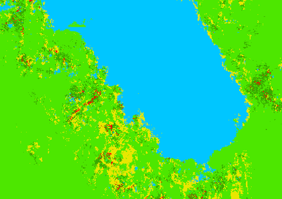
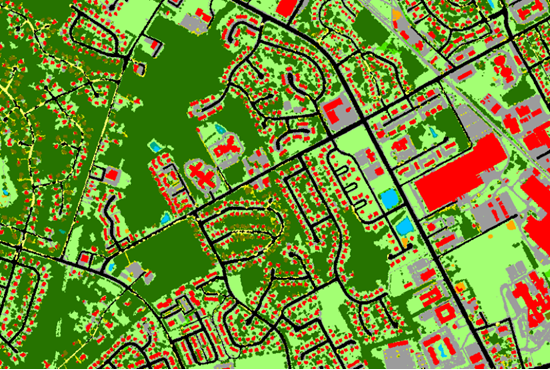
Use the Classify Pixels Using Deep Learning tool to classify imagery pixels. The tool runs a trained deep learning model on an input raster to produce a classified raster, with each pixel having an assigned class label. Land cover classification is a typical application for pixel classification. The image below is an example of land cover classification.
A typical pixel classification workflow using deep learning consists of three main steps:
- Create and export training samples. Create training samples using the Label Objects for Deep Learning pane, and use the Export Training Data For Deep Learning tool to convert the samples to deep learning training data.
- Train the deep learning model. Use the Train Deep Learning Model tool to train a model using the training samples you created in the previous step.
- Perform inferencing. Use the Classify Pixels Using Deep Learning tool. You will use the model you created in step 2.
For more examples, supported metadata formats, and model type architectures, see Deep learning model architectures.
Create and export training samples
Create a training schema and training samples, and export the training data.
If you have existing training samples in a raster dataset or a feature class, you can use the Export Training Data For Deep Learning tool and proceed to the Train a deep learning model section below.
- Create a training schema.
- Add the image to be used to generate the training samples to a map.
- In the Contents pane, select the image that you added.
- Click the Imagery tab.
- Click Deep Learning Tools, and click Label Objects for Deep Learning.
The Image Classification pane appears with a blank schema.
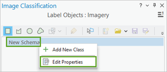
- In the Image Classification pane, right-click New Schema and click Edit Properties.
- Provide a name for the schema.

- Click Save.
- Add a new class to the schema.
- Right-click the schema you created, and choose Add New Class.
- Provide a name for the class.
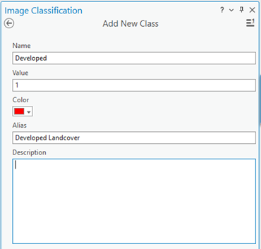
- Provide a value for the class.
The value cannot be 0.
- Optionally, choose a color for the class.
- Click OK.
The class is added to the schema in the Image Classification pane.
- Optionally, repeat steps 2a through 2e to add more classes.
- Create training samples.
- In the Image Classification pane, select the class you want to create a training sample for.
- Choose a drawing tool, such as Polygon.
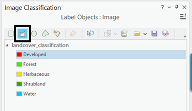
- Draw a polygon around the pixels that you want to represent the class you created.
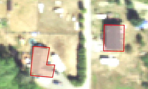
A new record is added to the Labeled Objects group in the Image Classification pane.
- Repeat steps 3a through 3c to create training samples for all the classes in the schema.
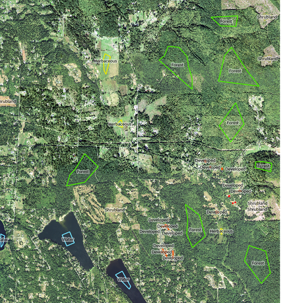
- When you finish creating samples, click Save in the Image Classification pane.
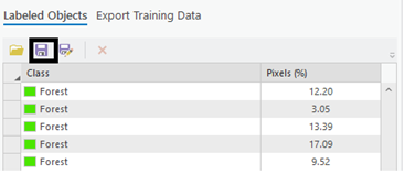
- In the Save current training sample window, browse to the geodatabase.
- Provide a name for the feature class, and click Save.
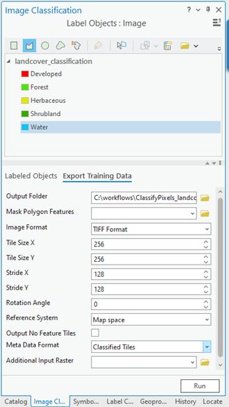
Before you can train the model, you must export the training samples as image chips. An image chip is a small image that contains one or more objects to be detected. An image chip is created and labeled for each training sample for the classes in the schema.
- In the Image Classification pane, click the Export Training Data tab.
- Provide the Output Folder value.
This is the path and name of the folder where the output image chips and metadata will be stored.
- Optionally, choose the Meta Data
Format value.
The Classified tiles option is the best format for multiband raster input. If the input is a multidimensional raster and you want to use the PSETAE model architecture, specify the RCNN Masks option.
- Click Run to export the training data.
- Provide the Output Folder value.
Train a deep learning model
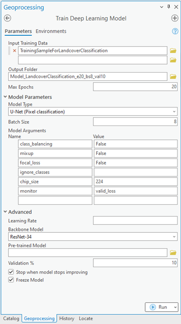
The Train Deep Learning Model tool uses the labeled image chips to determine the combinations of pixels in each image to represent the object. You will use these training samples to train a deep learning model. In the tool, only the Input Training Data and Output Model parameters are required.
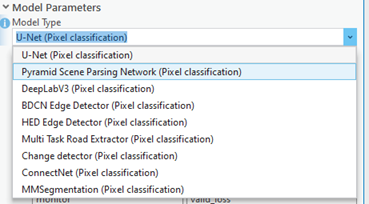
When you input the training data, an appropriate Model Type value is determined based on the Metadata Format value. For example, if the Classified tiles metadata format is specified, the U-Net option is specified for the Model Type parameter. The Model Type drop-down list is also updated with the model types that support the Classified tiles metadata format.
To train a deep learning model, complete the following steps:
- Open the Train Deep Learning Model tool.
- For the Input Training Data parameter, browse to and select the training data folder where the image chips are stored.
- For the Output Model parameter, provide the file path and name of the folder where the output model will be saved after training.
- Optionally, specify a value for the Max Epochs parameter.
An epoch is a full cycle through the training dataset. During each epoch, the training dataset you stored in the image chips folder is passed forward and backward through the neural network one time. Generally, 20 to 50 epochs are used for initial review. The default value is 20. If the model can be further improved, you can retrain it using the same tool.
- Optionally, change the Model Type parameter value in the drop-down list.
The model type determines the deep learning algorithm and neural network that will be used to train the model, such as the U-Net model architecture. For more information about models, see Deep Learning Models in ArcGIS . For documentation examples, supported metadata, and model architecture details, see Deep learning model architectures.
- Optionally, change the Model Arguments parameter value.
The Model Arguments parameter is populated with information from the model definition. These arguments vary depending on the model architecture that was specified. A list of model arguments supported by the tool are available in the Model Arguments parameter.
- Optionally, set the Batch Size parameter value.
This parameter determines the number of training samples that will be trained at a time. A batch size value can be determined by various factors such as number of image chips, GPU memory (if GPU is used), and learning rate, if a custom value is used. Typically, the default batch size produces good results.
- Optionally, provide the Learning Rate parameter value.
If no value is provided, the optimal learning rate is extracted from the learning curve during the training process.
- Optionally, specify the Backbone Model parameter value.
The default value is based on the model architecture. You can change the default backbone model using the drop-down list.
- Optionally, provide the Pre-trained Model parameter value.
A pretrained model with similar classes can be fine-tuned to fit the new model. The pretrained model must have been trained with the same model type and backbone model that will be used to train the new model.
- Optionally, change the Validation % parameter value.
This is the percentage of training samples that will be used to validate the model. This value depends on various factors such as the number of training samples and the model architecture. Generally, with a small amount of training data, 10 percent to 20 percent is appropriate for validation. If there is a large amount of training data, such as several thousand samples, a lower percentage such as 2 percent to 5 percent of the data is appropriate for validation. The default value is 10.
- Optionally, check the Stop when model stops improving parameter.
When checked, the model training stops when the model is no longer improving regardless of the Max Epochs value specified. The default is checked.
- Optionally, check the Freeze Model parameter.
This parameter specifies whether the backbone layers in the pretrained model will be frozen, so that the weights and biases remain as originally designed. If you check this parameter, the backbone layers are frozen, and the predefined weights and biases are not altered in the Backbone Model parameter. If you uncheck this option, the backbone layers are not frozen, and the weights and biases of the Backbone Model parameter value can be altered to fit the training samples. This takes more time to process but typically produces better results. The default is checked.
- Click Run to start the training.
Perform inferencing
Use the resulting deep learning model to perform pixel classification on an image. Inferencing is the process in which information learned during the deep learning training process is used to classify similar pixels in the image. Use the Classify Pixels Using Deep Learning tool since you are performing a pixel classification workflow.
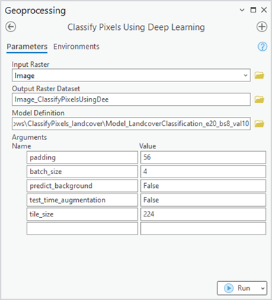
- Open the Classify Pixels Using Deep Learning tool.
- For the Input Raster parameter, browse to and select the input raster data you want to classify.
The input can be a single raster dataset, multiple rasters in a mosaic dataset or an image service, a folder of images, or a feature class with image attachments.
- For the Output Raster Dataset parameter, provide a name for the output dataset.
The output dataset will contain each valid pixel having an assigned class label in the input image.
- Specify the Model Definition value (*.emd or *.dlpk).
This is the model file that contains the training output. This is the output of the train deep learning section.
- For the Arguments parameter, accept the default values or modify them.
The Arguments parameter is populated with information from the Model Definition parameter. These arguments vary depending on the model architecture that was specified. In this example, the U-Net model architecture is used, so the following arguments are populated.
- padding—The number of pixels at the border of image tiles from which predictions are blended for adjacent tiles. Increase the value to smooth the output, which reduces artifacts. The maximum value of the padding can be half the tile size value.
- batch_size—The number of image tiles processed in each step of the model inference. This is dependant on the memory size of the graphics card.
- predict_background—Specify whether the background is classified. If set to true, the background class is also classified.
- test_time_augmentation—Test time augmentation is performed while predicting. If true, the predictions of flipped and rotated variants of the input image are merged into the final output.
- Click Run to start the inferencing.
The resulting classified raster is shown below.
