Join data spatially

A join operation adds fields from one data table (the join table) to another (the target table). The target table is typically a layer attribute table, and the purpose of the join is to symbolize the layer, query it, get statistics, or perform other analysis using information from the join table. A join can be temporary and be removed when you no longer need it, or it can be permanent.

There are two kinds of joins: attribute and spatial. An attribute join is based on a common field of values that exists in both tables. The common field ensures that records in the join table are matched correctly with records in the target table. A spatial join is based on a spatial relationship, such as containment or intersection, between features in two layers. Records in the join and target tables are matched according to the spatial relationship of their corresponding features.

In an attribute join, the join table can be a stand-alone (nonspatial) table or a layer attribute table. In a spatial join, both tables must be layer attribute tables.

Joins are one of many ways to combine data in ArcGIS Pro. You can add features from one dataset to another with the Append tool, combine datasets with the Merge tool, and create new data by spatially comparing datasets with overlay tools such as Intersect and Union.

Overview

• Video length: 11:25.
• This video was created with ArcGIS Pro 3.3.

The earthquake that struck Christchurch, New Zealand, on February 22, 2011, did enormous damage to the city's infrastructure. In the aftermath of the quake, engineering assessments were made of the area to determine requirements for repair and rebuilding.

In this tutorial, you'll look at historic places in the Christchurch urban area in relation to a layer of liquefaction risk. Liquefaction is a process in which sediment loses strength and stability during ground shaking, significantly increasing the potential for damage to buildings. You'll spatially join the liquefaction risk layer to the historic places layer to assign the appropriate risk value to each historic place.

After spatially joining the layers, you'll append new features to the historic places layer and update their liquefaction risk values.

• Estimated time: 60 minutes
• Software requirements:
  • ArcGIS Pro Basic

Note:

The quick-start tutorials are updated at each software release. For the best experience, use an online help version that matches your software version.

Open the project

You'll open a project from a project package on ArcGIS Online.

1. Start ArcGIS Pro and sign in if necessary.
2. Open a browse dialog box to search for the project in one of the following ways:
   • On the start page, click Open another project .
   • In an open project, click the Project tab on the ribbon. In the list of side tabs, click Open. On the Open page, click Open another project .

   

3. On the Open Project browse dialog box, in the navigation pane, under Portal , click ArcGIS Online .

   Note:

   If you are signed in to ArcGIS Enterprise , you must set your active portal to ArcGIS Online to access the tutorial data. If you can't do this, you can download the data from a browser.

4. At the top of the dialog box, in the Search box, type Join data spatially and press the Enter key.
5. In the list of search results, click Join data spatially to select the project package.

   Note:

   If there is more than one project package with this name, select the package with the Authoritative badge . In the Owner column, the owner name is ArcGISProTutorials. If you don't get any results, see No search results are returned.

6. Click OK.

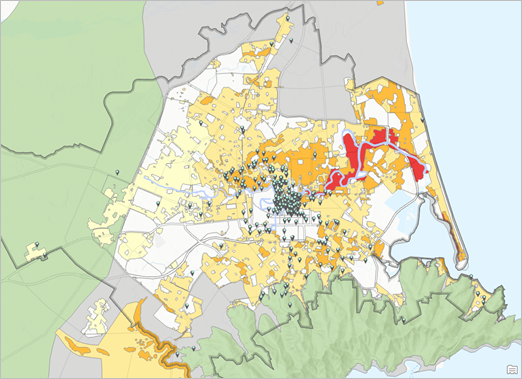
   The project opens with a map showing the urban area of Christchurch, New Zealand.

   

7. On the ribbon, click the View tab. In the Windows group, click Reset Panes and click Reset Panes for Mapping (Default).

   This ensures that the Contents and Catalog panes are open and that other panes are closed.

View the data

You'll examine the attributes of the Historic Places and Liquefaction Risk layers.

1. In the Contents pane, right-click the Historic Places layer and click Attribute Table .

   The attributes include each feature's name, address, and a historic registry number in the RegID field. At the bottom of the table view, you can see that there are 322 records in the layer.

2. In the Contents pane, right-click the Liquefaction Risk layer and click Attribute Table .

   The attributes for this layer include a risk category and the dates that the risk assessment was made and last modified.

   In the Category field, the three technical category values represent increasing risk of damage to buildings by liquefaction in a future earthquake.

   • Technical Category 1 represents a minimal risk of damage.
   • Technical Category 2 represents a slight to moderate risk of damage.
   • Technical Category 3 represents a moderate to significant risk of damage.

   Depending on the risk, different construction requirements may apply. In the red zone, where the risk is extreme, no construction is permitted. Risk has not been evaluated in nonresidential areas or in areas designated as needing assessment.

3. Close both open tables.
4. In the Contents pane, confirm that the Liquefaction Risk layer is selected. Press the Ctrl key and click the Historic Places layer.

   Both layers are selected.

5. On the ribbon, click the Map tab. In the Navigate group, click the Explore tool drop-down arrow and click Selected in Contents.

   When you click a location on the map, a pop-up will show the attribute values of features in the selected layers.

6. At the bottom of the map view, click the map scale drop-down arrow and click 1:10,000 so that historic places are easier to distinguish.
7. On the map, click a historic place.

   

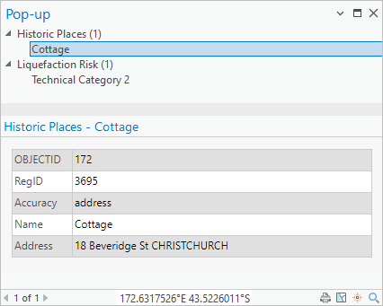
   The pop-up displays the attributes of the historic place and the risk polygon that contains it.

   Tip:

   At the top of the pop-up, you see the display value, or primary attribute, for the features in both layers. In this example, a feature named Cottage is selected and its attributes are shown at the bottom of the pane. To see the attributes of the liquefaction risk feature, click the value under Liquefaction Risk at the top of the pop-up.

8. Click a few more historic place features, then close the Pop-up pane.

   The pop-up shows the information of interest: the risk category associated with each historic place. However, clicking features one at a time is not the most efficient way to get this information. With a spatial join, you can add the liquefaction risk attributes to the Historic Places layer.

9. In the Contents pane, click the Historic Places layer to make it the only selected layer. Right-click the layer and click Zoom To Layer .

Join layers spatially

You'll join attributes from the Liquefaction Risk layer to the Historic Places layer according to the risk zone that each historic place is in.

1. In the Contents pane, right-click the Historic Places layer, point to Joins and Relates, and click Add Spatial Join .

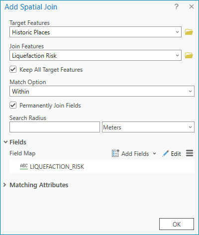
   The Add Spatial Join tool opens in a floating window. The Target Features parameter is correctly set to the Historic Places layer.

2. Click the Join Features drop-down arrow and click Liquefaction Risk.

   Attributes from this layer will be joined to the Historic Places table.

3. Click the Match Option drop-down arrow and click Within.

   Each historic place will get the attributes of the liquefaction risk polygon it lies within. (In this case, the default match option of intersection would also work because a feature that is within another feature also intersects it.)

4. Check the Permanently Join Fields check box.

   When the box is not checked (the default setting), the spatial join exists only in the current map and can be removed at any time. The source data of the target dataset is not modified. When the box is checked, the joined attributes modify the source data of the target dataset.

   You'll make the join permanent because later in the tutorial you'll append more features to the Historic Places layer. This can't be done when there is a temporary join on the layer.

   Tip:

   The Spatial Join tool can also be used for this workflow. The Spatial Join tool creates a new feature class with the attributes of the target and join features. The input datasets are not changed. In this tutorial, Add Spatial Join is used instead so that you can perform the join without creating a new output dataset.

5. Expand the Fields heading.

   The field map parameter displays a list of the fields in the Liquefaction Risk layer. The CATEGORY field is the only one of these fields you need to add to the Historic Places layer. You'll remove the others.

6. In the list of fields, click the CREATEDDATE field to select it. Press the Shift key and click the Shape_Area field.

   Four fields are selected.

7. Click Remove .

   

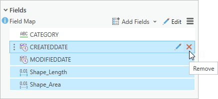
   The selected fields are removed, leaving only the CATEGORY field.

   In the Liquefaction Risk layer, the meaning of the CATEGORY field is clear. In the context of historic places, however, its meaning is not obvious: the category values might represent any number of things. You'll rename the field before running the tool. (The original name will remain in the Liquefaction Risk table.)

8. In the field map parameter, click Edit .

   The Field Properties dialog box appears. At the top, under Properties, you see the properties of the CATEGORY field, such as its name, alias, and type.

9. In the Field Name cell, highlight the existing value (CATEGORY) and replace it with LIQUEFACTION_RISK. Press the Enter key.
10. In the Alias cell, highlight the existing value and replace it with Liquefaction Risk. Press the Enter key.

    

    The alias is a display name that appears by default in the attribute table and in most geoprocessing contexts. An alias can include spaces; a field name cannot.

11. Click OK on the Field Properties dialog box.

    

12. Click OK to run the Add Spatial Join tool.
13. When the operation is completed, in the Contents pane, right-click the Historic Places layer and click Attribute Table .

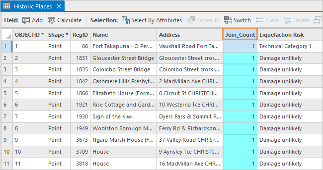
    The renamed Category field from the Liquefaction Risk layer is added to the table and displays its Liquefaction Risk alias. Each historic place is now associated with the risk category of the polygon in which it lies. A Join_Count field is also added. The value in this field is 1 for every record because each historic place is associated with exactly one risk polygon.

    You'll delete the Join_Count field, which you don't need.

14. In the Historic Places table, click the Join_Count field heading to select the field.

    

15. Right-click the selected field heading and click Delete .
16. On the Delete Field prompt, click Yes.

    Leave the Historic Places table open.

    Tip:

    You can also hide fields in a table to make them invisible without deleting them.

    Tip:

    Optionally, you can drag the table by its view tab to a new location that provides more viewing space for the map. For example, if you have two monitors, you can float the table outside the ArcGIS Pro window.

17. On the Quick Access Toolbar, click Save Project .

Evaluate the results

You'll open a Data Engineering view of the Historic Places table to view statistics for the joined table and to create a chart.

1. In the Historic Places table, click the Liquefaction Risk field heading to select the field.
2. Right-click the selected heading and click Explore Statistics .

   

   A Data Engineering view of the table opens and displays statistics for the LIQUEFACTION_RISK field:

   • The Count value is 322 (100%). This confirms that a liquefaction risk value exists for each historic place.
   • There are six unique values. The Liquefaction Risk table actually contains seven unique values. This means that there are no historic places in one of the risk categories. (Fortunately, it's the red zone.)
   • The mode, or most common value, is Nonresidential area.
   • The least common value is Technical Category 1.

3. In the Data Engineering view, hover over the Chart Preview column.

   

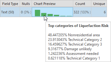
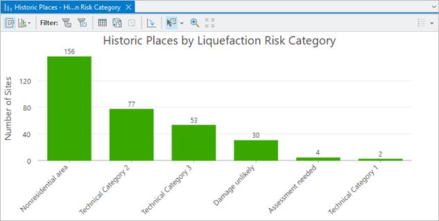
   The ScreenTip gives a percentage breakdown of the values. About half the historic places lie in nonresidential areas, about a quarter are in Technical Category 2, and so on.

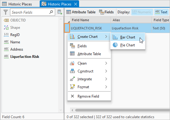
4. Right-click the row header (the square at the left edge of the row), point to Create Chart , and click Bar Chart .

   

   A chart view and the Chart Properties pane appear. The chart displays the number of historic places in each risk category. You'll modify its properties to make the chart easier to interpret.

   

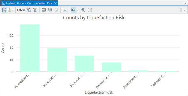
   The y-axis values and the orientation of the category labels may be different depending on the size of your chart view.

5. At the top of the Chart Properties pane, confirm that the Data tab is selected.
6. Under Data Labels, check the Label bars check box.

   On the chart, the number of historic places in each risk category appears above each bar.

7. At the top of the pane, click the Axes tab.
8. In the Label character limit box, change the value from 11 to 20. (You can use the arrow key or type the value and press the Enter key.)

   On the x-axis, the category values display their full names. By default, the label orientation is adjusted to best fit the available space. However, you may want to change the orientation.

9. Optionally, click the Label orientation drop-down arrow and choose a setting that you like.
10. At the top of the pane, click the General tab. (If you don't see it, click the options button and click General in the drop-down list.)
    1. In the Chart title box, delete the default title and type Historic Places by Liquefaction Risk Category. Press the Enter key.
    2. Uncheck the X axis title check box.
    3. In the Y axis title box, delete the default title and type Number of Sites. Press the Enter key.

    You may want to change the color of the bars, which is currently set to a light green.

11. Optionally, click the Series tab.
    1. In the Symbol column, click the light green color square.
    2. On the color palette that appears, click any color you like.
    3. Click outside the color palette to close it.

    

12. Click a bar on the chart to select it.

    On the map, the corresponding features in the Historic Places layer are selected.

13. Click a different bar to change the selection. Press the Ctrl key and click another bar to add to the selection.
14. In the chart view toolbar, click Clear Selection .
15. Close the chart view and close the Chart Properties pane. Leave the Data Engineering view open.

    In the Contents pane, the chart appears under the Historic Places layer. The chart doesn't exist independently of the layer: if you remove the layer from the map, or delete the map from the project, the chart will be gone. You can export a chart to save it as a graphics file.

16. On the Quick Access Toolbar, click Save Project .

Create a layer from a table

Data may become available that is relevant to a dataset you already have but that is stored in a different file. Suppose, for example, that you discover a .csv file with information about a couple of historic sites in Christchurch. If these sites are not already included in the Historic Places layer, you want to add them.

You'll add the .csv file as a table to the map. Because the file includes the spatial coordinates of the sites, you can create a layer from the table with features at the coordinate locations.

1. Make the Catalog pane active. At the top of the pane, ensure the Project tab is selected.
2. Expand the Folders container . Expand Join_data_spatially > commondata > userdata.

   The userdata folder contains a file named Christchurch Heritage Sites.csv.

3. Right-click Christchurch Heritage Sites.csv and click Add To Current Map .

   In the Contents pane, the file is added as a table under the Standalone Tables heading.

4. In the Contents pane, right-click Christchurch Heritage Sites.csv and click Open .

   

   The table contains information about two heritage sites, including a name, an address, a register number, and other fields.

5. Make the Historic Places table active by clicking its view tab.

   This table also contains name and address fields. The RegID field corresponds to the RegisterNumber field in the Christchurch Heritage Sites table. Although the field names are different, they store the same information.

6. Make the Christchurch Heritage Sites.csv table active again.

   The table includes X and Y fields with latitude-longitude coordinates in decimal degrees. You'll use these coordinates to create a layer from the table. Once you do that, you can see whether the features already exist in the Historic Places layer.

7. In the Contents pane, under Standalone Tables, right-click Christchurch Heritage Sites.csv, point to Create Points From Table and click XY Table To Point .

   The XY Table To Point tool opens in a floating window.

   The Input Table parameter defaults correctly to Christchurch Heritage Sites.csv. The X Field and Y Field parameters default correctly to the X and Y fields in the table. The Coordinate System parameter defaults to GCS_WGS_1984. Most latitude-longitude values are stored in this system, which makes this the best choice if you don't have additional information.

   Tip:

   Ideally, the file has metadata that identifies the coordinate system. You can confirm that the setting is correct for this file by right-clicking it in the Catalog pane and clicking View Metadata .

8. In the Output Feature Class text box, delete the entire path. In the empty box, type memory\Sites.

   

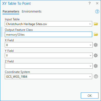
   You'll create the point features in a temporary memory workspace because you don't need to create output data. If it turns out that the features already exist in the Historic Places layer, you can discard this new layer. If they don't yet exist, you want to append them to the Historic Places layer. Either way, you don't need to save them to a new dataset.

   The path name memory\ specifies that the output is written to the memory workspace rather than to a feature class. When you end your ArcGIS Pro session, the memory workspace is cleared. The name Sites can be any name that you choose, but cannot include spaces.

9. Click OK.

   When the tool finishes, a layer named Sites is added to the top of the Contents pane.

10. In the Contents pane, right-click the Sites layer and click Zoom To Layer .

    You'll make the default symbols larger so they're easier to see.

11. In the Contents pane, click the symbol for the Sites layer

    The Symbology pane appears with formatting options for point symbols.

12. On the Gallery tab, in the list of symbols under ArcGIS 2D, click the Circle 3 symbol to select it.

    

    The symbol is updated on the map and in the Contents pane.

13. In the Contents pane, turn the Sites layer off, then turn it on again.

    You can see that features do not already exist in the Historic Places layer at these locations.

Append data

You'll append the two features from the Sites layer to the Historic Places layer using the Append tool. Because the tables in the two layers have different schema, you need to match some fields manually. You'll do this with the field map parameter you used earlier.

Tip:

Another option is to copy features from one layer to another with the Copy and Paste Special commands on the Edit tab of the ribbon. For a small number of features, this can be a useful approach. The copy and paste workflow also supports field mapping through the configuration of editor settings.

1. Make the Historic Places Data Engineering view active.
2. Right-click the row header (the square at the left edge of the row), point to Integrate , and click Append .

   The Append tool opens in a floating window. A message at the top of the dialog box alerts you that the tool modifies the target dataset (rather than creating new output data).

3. Click the Input Datasets drop-down arrow and click Sites.

   The target dataset is correctly set to Historic Places by default.

4. Click the Field Matching Type drop-down arrow and click Use the field map to reconcile field differences.

   

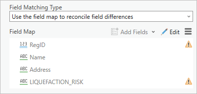
   The dialog box expands to show the field map parameter.

   The RegID and LIQUEFACTION_RISK fields are marked with warning icons because they don't have fields with the same name in the input dataset. (For this reason, the tool will fail if you run it with the default setting that input fields must match target fields.)

   As you saw earlier, the RegisterNumber field in the Sites table and the RegID field in the Historic Places table both contain historic registry numbers. When the field names differ but the values are related, you can manually match those fields using the field map.

5. In the field map parameter, click Edit .

   The Field Properties dialog box appears.

6. On the Field Properties dialog box, in the Fields list, confirm that the RegID field is selected (highlighted in blue). Scroll through the input fields list and click the RegisterNumber field.

   

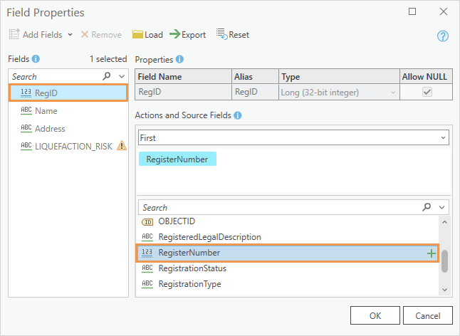
   Under Actions and Source Fields, the RegisterNumber field appears as a tag, indicating it is matched to the RegID field as a source field. The warning icon is removed from the RegID field.

   You'll leave the LIQUEFACTION_RISK field unmatched because it doesn't have a corresponding field in the Sites table. When the tool runs, two new records will be added to the Historic Places table. Attributes will be processed as follows:

   • For matching fields, values in the Sites table will be added to the corresponding field in the Historic Places table. For example, addresses will be added to the Address field and registry numbers will be added to the RegID field.
   • Fields in the Historic Places table that don't have a matching field will have null values for the appended records. This means that the LIQUEFACTION_RISK field will have null values.
   • Fields in the Sites table that don't have a matching field will not be added to the Historic Places table. These include the DateRegistered and LocalAuthorityName fields, and several others.

   Note:

   As you saw earlier, the spatial coordinates of the two heritage sites are in decimal degrees. The Append tool will automatically project these coordinates to the coordinate system of the target dataset, which is NZGD 2000 New Zealand Transverse Mercator.

7. Click OK on the Field Properties dialog box.

   The Append tool is one of several geoprocessing tools that allows you to undo geoprocessing results. In this tutorial, you will leave the Enable Undo toggle button turned off, but you may want to use it in other circumstances.

8. Click OK on the Append tool.
9. When the tool finishes, make the Historic Places attribute table active.

   At the bottom of the table view, you see that there are now 324 records in the table (two more than before).

10. At the bottom of the table view, click Move to End to go to the end of the table.

    

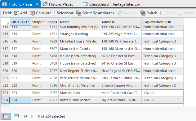
    The two records from the Sites layer have been added to the table. As expected, the Liquefaction Risk field has null values for these records.

11. Make the Christchurch Urban Area map view active. In the Contents pane, turn the Sites layer off.

    

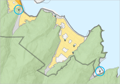
    The appended features appear on the map in the correct locations. You no longer need the Sites layer.

12. In the Contents pane, right-click the Sites layer and click Remove .

    To finish your work, you'll identify the liquefaction risk values for the new features and add them to the table.

13. On the Quick Access Toolbar, click Save Project .

Identify risk zones for the new features

The new features were added after the spatial join and therefore have null values in the Liquefaction Risk field. You'll use the Explore tool to find the values for these features.

1. On the ribbon, on the Map tab, click the Explore tool drop-down arrow and click Visible Layers.
2. On the map, click the new feature in the Historic Places layer that represents Moncks Cave. (Of the two new features, this is the one farther north.)

   

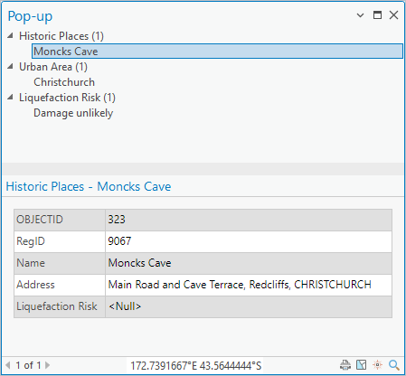
   On the pop-up, you see that Moncks Cave lies in a liquefaction risk zone in which damage is unlikely.

3. Move the pop-up out of the way if necessary. On the map, click the new feature for the Rotten Row Baches.

   This feature lies in a nonresidential area.

   Note:

   If the Liquefaction Risk layer doesn't appear in the pop-up, zoom in on the feature and click it again. The feature lies at the edge of the layer extent. If you click outside the extent, you won't get a result.

4. Close the Pop-up pane.
5. On the ribbon, on the Map tab, click the Explore tool drop-down arrow and click Topmost Layer to restore the default setting.

Calculate field values

Field calculations update table values on the basis of an expression you write. In this case, you only need to update two values and you could edit the table cells manually. However, in cases in which you need to update hundreds or thousands of values, field calculations are essential. Using field calculations also minimizes the risk of data entry mistakes.

1. Make the Historic Places attribute table active. In the table, click the number 323 row header (the gray square at the left edge of the row) to select the record for Moncks Cave.
2. Right-click the Liquefaction Risk field heading and click Calculate Field .

   The Calculate Field dialog box appears. A message at the top of the dialog box alerts you that the tool modifies the input table.

   The Input Table parameter defaults to Historic Places. The toggle button indicates that values will be calculated for the selected record only. The Field Name (Existing or New) parameter defaults to Liquefaction Risk. The Expression Type parameter defaults to Python.

   You'll define the expression to calculate. You want to replace the current null value for Moncks Cave with the Damage unlikely value.

3. In the Fields list, click Liquefaction Risk to select it. Click the Insert Values drop-down arrow and click Damage unlikely.

   

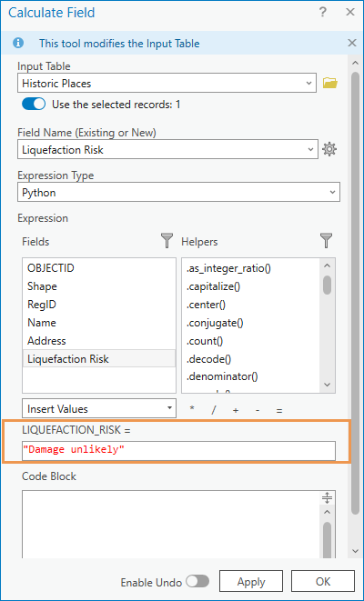
4. Click OK.

   In the Historic Places table, the null value for Moncks Cave is updated.

5. In the table, click the number 324 row header to select the record for Rotten Row Baches.
6. Right-click the Liquefaction Risk field heading and click Calculate Field .

   As before, the Input Table and Field Name (Existing or New) parameters default correctly. You need to change the expression, which defaults to the one you set previously.

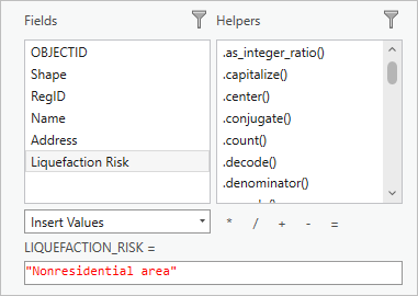
7. In the expression box, delete the expression "Damage unlikely".
8. In the Fields list, click Liquefaction Risk to select it. Click the Insert Values drop-down arrow and click Nonresidential area.

   

9. Click OK.

   In the Historic Places table, the null value for Rotten Row Baches is updated.

   This completes your work. Each historic place has a liquefaction risk value that can be used to evaluate safety requirements for maintaining and rebuilding the sites. On your own, you may want to go on and symbolize the Historic Places layer with unique values based on liquefaction risk or create a table of summary statistics.

10. On the toolbar at the top of the table view, click Clear to clear the selected record.
11. Close the open tables and the Data Engineering view.
12. In the Contents pane, right-click the Historic Places layer and click Zoom To Layer .
13. On the Quick Access Toolbar, click Save Project .

In this tutorial, you used a spatial join to add an earthquake liquefaction risk attribute from a polygon layer to a point layer of historic sites. You explored the properties of the joined table in a Data Engineering view. You converted a .csv file to a map layer and appended features from this layer to the layer of historic sites. Finally, you calculated values for the appended records to fill in missing information.

To get more experience with spatial joins, see the Get started with ArcGIS Pro and Borrow attributes with a spatial join tutorials. Learn more about Data Engineering in the Data Engineering in ArcGIS Pro series of articles and tutorials. To learn how to append new data to a layer while updating its existing data, see the article Upsert your datasets using the Append tool in ArcGIS Pro.