With a lot of spatial data analysis, the scale of the analysis is important. The default value for the Conceptualization of Spatial Relationships parameter of the Hot Spot Analysis tool, for example, is a fixed distance band. For many density tools, you need to provide a radius value. The distance you provide should relate to the scale of the question you are trying to answer or to the scale of remediation you are considering. For example, you want to understand childhood obesity. What is the scale of analysis? Is it at the individual household or neighborhood level? If so, the distance you use to define the scale of the analysis will be small, encompassing the homes within a block or two of each other. Alternatively, what will be the scale of remediation? Maybe the question involves where to increase after-school fitness programs as a way to potentially reduce childhood obesity. In that case, the distance will likely be reflective of school zones. Sometimes it’s fairly easy to determine an appropriate scale of analysis; if you are analyzing commuting patterns and know that the average journey to work is 12 miles, for example, 12 miles is an appropriate distance to use for the analysis. Other times it is more difficult to justify any particular analysis distance. This is when the Incremental Spatial Autocorrelation tool is helpful.
Whenever you see spatial clustering in the landscape, you are seeing evidence of underlying spatial processes at work. Knowing something about the spatial scale at which those underlying processes operate can help you select an appropriate analysis distance. The Incremental Spatial Autocorrelation tool runs the Spatial Autocorrelation (Global Moran’s I) tool for a series of increasing distances, measuring the intensity of spatial clustering for each distance. The intensity of clustering is determined by the z-score returned. Typically, as the distance increases, so does the z-score, indicating intensification of clustering. At a particular distance, however, the z-score generally peaks. Sometimes there are multiple peaks.

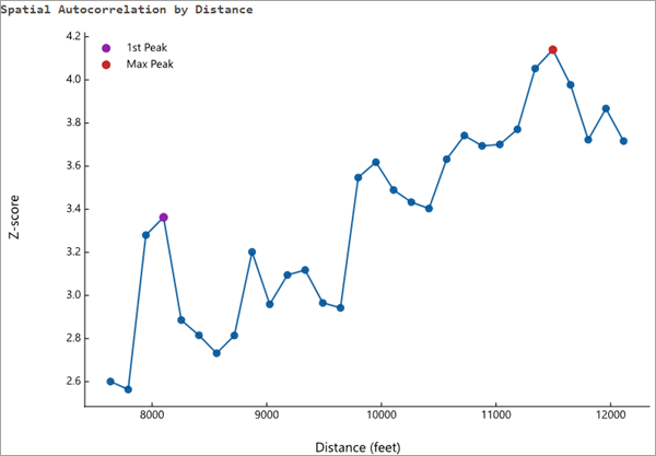
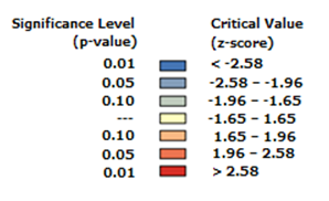
Peaks reflect distances where the spatial processes promoting clustering are most pronounced. The color of each point on the graph corresponds to the statistical significance of the z-score values.

One strategy for identifying an appropriate scale of analysis is to select the distance associated with the statistically significant peak that best reflects the scale of the question. Often this is the first statistically significant peak.
Determine the Beginning Distance and Distance Increment values
All distance measurements are based on feature centroids and the default Beginning Distance parameter value is the smallest distance that will ensure every feature has at least one neighboring feature. This is generally a good choice, unless the dataset includes locational outliers. Determine whether there are locational outliers; then select all but the outlier features and run Incremental Spatial Autocorrelation on only the selected features. If you find a peak distance for the selection set, use that distance to create a spatial weights matrix file based on all of the features (even the outliers). When you run the Generate Spatial Weights Matrix tool to create the spatial weights matrix file, set the Number of Neighbors parameter to a value so that all features will have at least that many neighboring features.
The default Increment Distance parameter value is the average distance to each feature's nearest neighboring feature. If you've determined an appropriate starting distance using the strategies above and still don't see a peak distance, you may want to experiment with smaller or larger increment distances.
No peak distance
In some cases, you may use the Incremental Spatial Autocorrelation tool and get a graph with a z-score that continues to rise with increasing distances; there is no peak. This most often happens in cases when data has been aggregated and the scale of the processes impacting the Input Field variable are smaller than the aggregation scheme. You can try making the Increment Distance value smaller to see if that captures more subtle peaks. Sometimes, however, there is no peak because there are multiple spatial processes, each operating at a different distance, in the study area. This is often the case with large point datasets that are noisy (no clear spatial pattern to the point data values you're analyzing). In this case, you need to justify the scale of analysis using other criteria.
Interpret the results
When you run the Incremental Spatial Autocorrelation tool, the z-score results for each distance are written as messages. To access the messages, hover over the progress bar, click the pop-out button, or expand the messages section in the Geoprocessing pane. You can also access the messages for a previously run tool through the geoprocessing history. When you specify a path for the optional Output Table parameter, a table is created that includes fields for Distance, Morans I, Expected I, variance, z_score, and p_value.
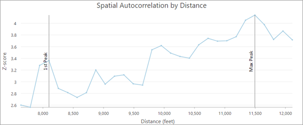
By examining the Spatial Autocorrelation by Distance line chart and z-score values written as messages, you can determine if there are any peak distances. In the image below, the chart has two peak z-scores associated with distances of 8100 and 11500 feet.

If you use the Output Table parameter to create a table of the autocorrelation values, the table includes the Spatial Autocorrelation by Distance line chart. This is the same chart that appears in the messages.
Additional resources
For additional information, see the following:
- Videos outlining best practices for performing a hot spot analysis:
- The Spatial Pattern Analysis Tutorial is an analysis of Dengue Fever data that uses the Incremental Spatial Autocorrelation tool.
- See Selecting a Fixed Distance Band in Modeling spatial relationships.
- How Hot Spot Analysis (Getis-Ord Gi*) works includes a discussion of finding an appropriate scale of analysis.
- For an up-to-date list of all of the spatial statistics resources available, go to the Spatial Statistics Resources page.