Mit der Geostatistical Analyst-Lizenz verfügbar.
When modeling the semivariogram, the autocorrelation can be examined and quantified. In geostatistics, this is called spatial modeling, also known as structural analysis or variography. In spatial modeling of the semivariogram, you begin with a graph of the empirical semivariogram, computed as,
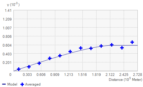
Semivariogram(distance h) = 0.5 * average [ (value at location i– value at location j)2]for all pairs of locations separated by distance h. The formula involves calculating half the difference squared between the values of the paired locations. To plot all pairs quickly becomes unmanageable. Instead of plotting each pair, the pairs are grouped into lag bins. For example, compute the average semivariance for all pairs of points that are greater than 40 meters but less than 50 meters apart. The empirical semivariogram is a graph of the averaged semivariogram values on the y-axis and distance (or lag) on the x-axis (see diagram below).

Again, it is the intrinsic stationarity assumption that allows replication. Thus, you can use averaging in the semivariogram formula above.
Once you've created the empirical semivariogram, you can fit a model to the points forming the empirical semivariogram. The modeling of a semivariogram is similar to fitting a least-squares line in regression analysis. Select a function to serve as your model, for example, a spherical type that rises at first and then levels off for larger distances beyond a certain range.
The goal is to calculate the parameters of the curve to minimize the deviations from the points according to some criterion. There are many different semivariogram models to choose from.