Service multiple customers from a single distribution center using Last Mile Delivery

Complexity: BeginnerData Requirement: ArcGIS Tutorial Data for Desktop

A breakfast sandwich start-up has taken off and turned into a thriving business delivering sandwiches to independent coffee shops throughout the San Francisco area. The sandwiches have gained a following of their own, and the coffee shops order them by the dozen. To work with the timing of the coffee rush hour, the sandwich company must deliver the sandwiches to the coffee shops between 5:00 a.m. and 7:30 a.m. This means the sandwich company and its fleet of drivers must be as efficient as possible in making their deliveries during this small time window.

For now, the drivers are not running into space issues for transporting all of the breakfast sandwiches, but they end up running behind schedule when delivering orders with bigger quantities. Since the time window for delivery is so important, the company wants to better account for the delivery time based on quantities being delivered.

Note:

The data used in this tutorial is fictitious and has been created solely to solve the example scenario stated above.

Get the data

The data for this tutorial is available for download.

1. Go to the data download page.
2. Click the Download button, and save the file locally.
3. Unzip the downloaded file.

Create a map

Complete the following steps to create a map:

1. Start ArcGIS Pro.
2. Create a new project by clicking the Map template. Optionally, change the name of your project and location.

   A new project with a map appears.

Add the tutorial data to the project

A network dataset is an intelligent model of the road system. It contains not only the location and attributes of roads but also information about how roads relate to one another, such as which roads are connected, which turns between connected roads are allowed or prohibited, and other information that affects what travel paths are possible and how long travel takes.

Note:

If you perform an analysis using ArcGIS Online, the solver references a high-quality, worldwide network dataset stored in the ArcGIS Online cloud and uses ArcGIS Online credits. You can also use your own network dataset stored locally on your machine or use ArcGIS Enterprise to publish routing services using your own network dataset and configure the services with your enterprise portal to consume them from ArcGIS Pro.

In this set of steps, add a network dataset to the map.

1. In the Catalog pane, which is on the right side of the application by default, right-click Folders and choose Add Folder Connection .

   The Add Folder Connection dialog box appears.

2. Browse to the folder where you placed the tutorial data, double-click Network Analyst, and click Tutorial to select the folder.
3. Click OK.

   A connection to the Tutorial folder is created.

Next, add the network dataset contained in the folder to the map.

4. In the Catalog pane, expand Folders > Tutorial > SanFrancisco.gdb > Transportation.
5. Drag Streets_ND, which has a network dataset icon , onto the map.

   The network dataset is added to the Contents pane and to the map.

6. In the Contents pane, uncheck Streets_ND to display the basemap only.

Geocode the coffee shops

You will now geocode the CoffeeShops.csv file to make a feature class with the customer locations. When a table has addresses for a location, it can be located on a map through geocoding. The addresses can be in a single field or in multiple fields of the table.

Note:

If you have your own street data, you can create a locator using that data; otherwise, Esri offers the ArcGIS World Geocoding Service, which consumes credits.

1. In the Catalog pane, browse to the location of the tutorial data, right-click SanFranciscoLocator.loc, and click Add to Project.
2. Right-click CoffeeShops.csv, and from the context menu, select Geocode Table.

   The Geocode Table pane appears.

3. In the Geocode Table pane, click Start.

   

4. From the Input Locator drop-down list, select SanFranciscoLocator.
5. In the Geocode Table pane, click Next.
6. Ensure that Input Table is pointing to CoffeeShops.csv; the drop-down list has More than one field as the address for the customers in the StreetAddress, City, and Postal fields;, and click Next.
7. Map the address fields as follows:
   • Address or Place to StreetAddress
   • City to City
   • ZIP to Postal
   • State to State
8. Click Next.

   Leave the Output as is to save it to the project workspace.

9. For Preferred Location Type, choose Routing Location from the drop-down options.

   This option places the located features on the street network location instead of the roof top. In Network Analyst, points are spatially located at the closest street edge. The center of a building can sometimes be closer to a street other than the driveway access street.

10. Leave Output Fields set to All, and click Next.
11. For Category, check Address, and click Finish.
12. Click Run.

    Once the process finishes, a message appears asking if you want to rematch.

13. Click No, since all the locations were matched correctly.

    

14. Close the Geocode Table pane.

Create the last mile delivery analysis layer

The Last Mile Delivery solver focuses on the subset of vehicle routing problems associated with delivering packages to end customers. Last Mile Delivery problems have a single distribution center from which delivery vehicles are dispatched to visit customer locations. This layer allows you to add information about the customers, starting and ending location for the routes, the vehicles, and the drivers. There are several feature classes and tables for gathering information. There are also several parameters you can access on the Last Mile Delivery Layer tab to ensure that it is solving for the correct date and using the correct units and vehicle travel information.

To create the last mile delivery analysis layer, complete the following steps:

1. On the Analysis tab, in the Workflows group, click Network Analysis > Last Mile Delivery .

   The Last Mile Delivery analysis layer is added to the Contents pane. It includes several sublayers that contain the inputs and outputs of the analysis.

   This layer is referencing the San Francisco network dataset because the network was in the Contents pane when the Last Mile Delivery layer was created.

   Note:

   To review or change the network data source that is used to create the network analysis layer, on the Analysis tab, in the Workflows group, click the Network Analysis drop-down menu and view Network Data Source.

Add orders

Orders are used to specify information about the customers. Each order can contain information about the amount of time the driver is expected to be at that location, the quantity of items being delivered or picked up, and appointment times, among other things.

To add orders, complete the following steps:

1. Select the Last Mile Delivery layer in the Contents pane to enable the tab.

   

2. Click the Last Mile Delivery Layer tab, and in the Input Data section, click the Import Orders button .

   The Add Locations dialog box appears.

3. Select CoffeeShops_Geocoded for Input Locations.
In steps 4 through 6, you will do a field mapping. This is to ensure that the information regarding the coffee shops from the CoffeeShops_Geocoded feature class is correctly mapped and populated to the matching fields in the Orders sublayer.
4. Under Field Mappings, select Name from the Property section.
5. From the Field Name drop-down list, select USER_Name near the bottom of the list.

   The Last Mile Delivery solver requires a unique name for each order. Since every coffee shop on the list for delivery has a unique name, the coffee shop names (in the USER_Name field) is mapped to the Name field on the Orders sublayer.

6. Map the following additional property as DeliveryQuantity_1 > USER_DozensOfBreakfastSandwiches.

   The sandwich shop is delivering sandwiches by the dozen. The quantity to be delivered to each shop is tracked in the USER_DozensOfBreakfastSandwiches field so this will be mapped to the DeliveryQuantity_1 field allowing the Last Mile Delivery solver to track the dozens of sandwiches delivered to each location.

7. Select CurbApproach from the Property section, and select Right side of vehicle from the Default Value drop-down list.

   The CurbApproach field designates the side of the street the location must be in relationship to the vehicle when servicing it. With these routes being in San Francisco, where cars drive on the right side of the street, setting CurbApproach to the right side of the vehicle ensures that the delivery van is parked at the curb next to the coffee shops, and the driver will not need to cross the road.

8. Click OK.

   The coffee shops are added to the Orders sublayer.

   

   A warning message appears indicating that the geocoding process made the Name field in the CoffeeShops_Geocoded feature class too long for the Name field in the Orders sublayer. Close the warning message window since the names were not too long.

   

You will now update the service time based on the delivery quantity.
9. In the Contents pane, right click the Orders sublayer, and select Attribute Table.
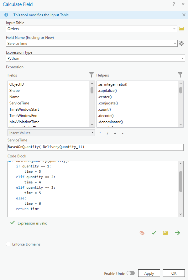
10. In the attribute table, right-click the ServiceTime field, and select Calculate Field.

    The Calculate Field dialog box appears.

In steps 11 and 12, you will calculate the service time based on the quantity of sandwiches a particular coffee shop ordered. The quantity ordered is by the dozen and the time it takes to deliver is in minutes. If the coffee shop ordered one, two, or three dozen sandwiches, it will take 3, 4, or 5 minutes, accordingly, to make the delivery. Any order above three dozen will take 6 minutes to deliver to the coffee shop.
11. Set the ServiceTime value to BasedOnQuantity(!DeliveryQuantity_1!).
12. Use the following for Code Block:

def BasedOnQuantity(quantity):
    if quantity == 1:
        time = 3
    elif quantity == 2:
        time = 4
    elif quantity == 3:
        time = 5
    else:
        time = 6
    return time

The window should resemble the following:



13. Click the check mark to verify the expression.
14. Click OK.

    The ServiceTime field is now populated with an appropriate value.

15. Close the attribute table.

Add the sandwich shop location to the Depots sublayer

Depots are where the routes start and end their day. All routes must start and end at the same location. For this analysis, the sandwich shop will be used as the depot. As with the customer data, the sandwich shop's address can be geocoded. However, since this is a single address, you will use the Locate pane instead to geocode the address and add it to the Depots sublayer.

Note:

Using the Add to Feature Class option with the ArcGIS World Geocoding Service consumes credits. Using the provided locator does not consume credits.

To add the sandwich shop location, complete the following steps:

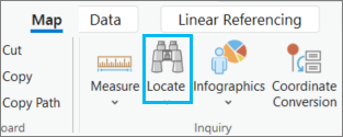
1. Click the Map tab, and in the Inquiry group, click the Locate button .

   

   The Locate pane appears.

2. Click the Options drop-down arrow next to the search box.

   

3. Check SanFranciscoLocator.
4. In the search text box, enter the sandwich shop’s address, 50 Southdale Ave. Daly City, CA 94015, and press Enter.
5. In the Locate pane, right-click option A, and select Add To Feature Class.

   The Add To Feature Class window appears, where you can select the feature class to add the address.

6. Expand Last Mile Delivery: Depots, select the Depots template, and click OK.
7. In the Contents pane, right-click the Depots sublayer, and select Attribute Table.

   A row has been added to the attribute table representing the only location of the sandwich shop. The full address of the sandwich shop was included as the depot's name.

8. Close the attribute table.
9. On the Edit tab, clear the selection and save the edits.
10. Close the Locate pane.

Add information to the Routes sublayer

Routes include information about both the vehicle and the driver. Information can be included about a driver's workday, such as when they start and how long they can work in a day. Vehicle information can also be included, such as capacity and the cost to operate it.

To efficiently deliver the orders to 173 coffee shops, set the following parameters while adding the routes. You will specify the number of routes that can service 173 coffee shops, the starting and ending location of the route (which is the location of the sandwich shop), the earliest time that the route can begin (the delivery time window is 5 a.m. to 7:30 a.m.), the capacity of the truck, the maximum total time the route can travel, and how much a driver is paid per hour.

To add routes and other information to the Routes sublayer, complete the following steps:

1. In the Contents pane, right-click the Last Mile Delivery group layer name, and select Zoom to Layer to zoom out to the full extent.
2. Return to the Last Mile Delivery Layer tab.
3. In the Input Data group, click the Import Routes drop-down list, and select Add Routes.

   The Add Vehicle Routing Problem Routes dialog box appears.

4. Set the following values:
   1. Number of Routes—12

      The sandwich shop has 12 vehicles for these deliveries so that is the number of routes they can send.

   2. Start Depot Name—50 Southdale Ave. Daly City, CA 94015

      The route must start and end at the sandwich shop, so both the Start Depot Name and End Depot Name values are the address of the sandwich shop.

      You can select Start Depot Name from the drop-down list and the value must match the value in the Name field of the Depots sublayer.

   3. End Depot Name—50 Southdale Ave. Daly City, CA 94015

      You can select End Depot Name from the drop-down list and the value must match the value in the Name field of the Depots sublayer.

   4. Earliest Route Start Time—5:00 am

      The routes must start at 5:00 a.m. to get the breakfast sandwiches to the coffee shops in time for the morning rush.

   5. Capacity_1—150

      Each vehicle can hold a maximum of 150 dozen breakfast sandwiches. It is important that the units used for Capacity_1 match the units for DeliveryQuantity_1, which in this case is dozen of sandwiches.

   6. Max Total Time—150

      The routes must be finished and back at the sandwich shop by 7:30 a.m. This gives the drivers 2.5 hours to complete their routes. Since the time field units being used to model this problem is minutes, you need to enter 150 minutes for Max Total Time.

   7. Cost Per Unit Time—0.5

      The drivers are paid $30 per hour, but since minutes are used to model this problem, it equals $0.5 per minute.

5. Click OK to run the tool.

   Twelve routes are added to the Routes sublayer.

Add zones

To keep drivers in their preferred regions of town, you will now add zones.

1. On the Last Mile Delivery Layer tab, in the Input Data section, click the Create Features button .
2. In the Create Features pane, select the Zones template.
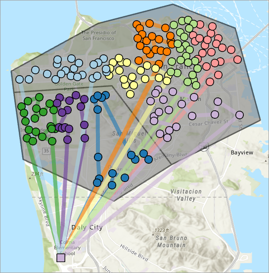
3. Draw two polygons to separate the north and south of Golden Gate Park and San Miguel Hills. The zones should resemble the image below.

   

4. In the Contents pane, right-click Zones, and select Attribute Table.
5. For the polygon south of Golden Gate Park and San Miguel Hills, change the Name field value to South.
6. For the polygon north of Golden Gate Park and San Miguel Hills, change the Name field value to North.
7. Open the Routes attribute table and scroll to the right to the ZoneName and IsHardZone fields.
8. Right click the IsHardZone field, and click Calculate Field.

   The Calculate Field dialog box appears.

9. Set the IsHardZone value to True.

   This setting defines that the routes can only deliver orders within the zone specified.

10. Select the first three rows in the attribute table, right-click ZoneName field, and click Calculate field.

    The Calculate Field dialog box appears.

11. Set the ZoneName value to South.

    This places a limit on the first three routes that can deliver orders in the southern zone only.

12. Switch the row selection in the attribute table and use Calculate field to set the ZoneName value to North for the remaining nine routes.

    This places a limit on the remaining nine routes that can deliver orders in the northern zone only.

13. Clear the selection and save the edits.
14. Close the attribute table.

Set the date and run the analysis

You will now set a date for when the routes will start. You don't need to set the time because each route has a time set from when you added routes using the Add Vehicle Routing Problem Routes tool in a previous section.

1. On the Last Mile Delivery Layer ribbon, in the Date and Time section, click the Default Date drop-down arrow and set the date as 03/14/2024.
2. In the Analysis group, click Run.

   The Last Mile Delivery layer solves. The orders are assigned to routes, and the symbology updates to show the routes and their assigned orders in matching colors.

   

3. In the Contents pane, right-click the Routes sublayer, and select Attribute Table.
4. Scroll to the right on the table to the OrderCount output field.
Review the results. Several feature classes in the Last Mile Delivery analysis layer have output fields that provide details about the solved solution. The Routes table provides an overview of each route, but you can also review details about each order. The Routes output includes the number of locations each driver goes to, the total time it takes, when the route starts, and when it is expected to return to the sandwich shop. You will notice that three routes did not service any of the coffee shops, because they were covered by other routes. Consequently, most of the fields for these three routes have null values.