Geoprocessing tools are essential for spatial analysis, but they have other uses as well. Spatial analysis includes activities such as comparing places, determining how places are related, finding best locations and paths, detecting patterns, and making predictions. Most geoprocessing tools work on an input dataset to create an output dataset. Some tools modify the attributes or geometry of an input dataset. A few tools have other effects, such as creating selections on layers or generating messages or reports.
Overview
- This video was created with ArcGIS Pro 3.5
In this tutorial, you'll use geoprocessing tools to solve a spatial problem.
- Estimated time: 45 minutes
- Software requirements: ArcGIS Pro Basic
Note:
The quick-start tutorials are updated at each software release. For the best experience, use an online help version that matches your software version.
Open the project
Nassella tussock is an invasive weed accidentally brought to New Zealand in the late 1800s. It is now well established in the Marlborough and Canterbury regions on the South Island. It spreads quickly, crowds out other grasses, and is hard to eradicate. It is unpalatable to livestock, which makes it a threat to pastoral farming. Nassella tussock seeds are spread mainly by wind, but also by animals, people, and vehicles.
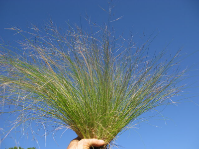
In this tutorial, you'll look for Nassella tussock growing near commercial campgrounds (campgrounds for motorhomes). Campers who come in contact with the weed during recreational activities may get seeds in their clothing or gear and take these seeds with them when they leave. If your analysis shows that Nassella tussock grows near commercial campgrounds, agriculture officials can provide information to help campers identify and avoid it.
The analysis has three parts. First, you'll create buffers, or proximity zones, around the commercial campgrounds. Next, you'll see which of these buffers contain Nassella tussock. Finally, you'll calculate the amount of Nassella tussock within the buffers.
- Start ArcGIS Pro and sign in if necessary.
- Open a browse dialog box to search for the project in one of the following ways:
- On the start page, click Open another project
 .
. - In an open project, click the Project tab on the ribbon. In the list of side tabs, click Open. On the Open page, click Open another project
 .
.

- On the start page, click Open another project
- On the Open Project browse dialog box, in the navigation pane, under Portal
 , click ArcGIS Online
  .
.Note:
If you are signed in to ArcGIS Enterprise
 , you must set your active portal to ArcGIS Online to access the tutorial data. If you can't do this, you can download the data from a browser.
 - At the top of the dialog box, in the search box, type Use geoprocessing tools and press the Enter key.
- In the list of search results, click Use geoprocessing tools to select the project package.
Note:
If there is more than one project package with this name, select the package with the Authoritative badge
 . In the Owner column, the owner name is ArcGISProTutorials. If you don't get any results, see No search results are returned.
 - Click OK.
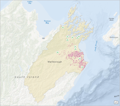
The project opens to the Marlborough region of New Zealand. Commercial campgrounds are displayed along with the known distribution of Nassella tussock.
The Nassella Tussock Range layer does not represent the density of the plant at a given location. A marked area may be heavily infested or may have only scattered plants.
Open the Geoprocessing pane
To carry out the analysis, you'll run tools from the Geoprocessing pane. First, you'll see how these tools are organized in ArcGIS Pro.
- On the ribbon, click the View tab. In the Windows group, click Pane Sets
 and click Geoprocessing
  .
.This ensures that the Contents, Catalog, and Geoprocessing panes are open and that other panes are closed. In the Geoprocessing pane, on the Favorites tab, some common geoprocessing tools are readily accessible.
Tip:
You can access the Geoprocessing pane without resetting panes. To do so, on the Analysis tab on the ribbon, in the Geoprocessing group, click Tools
 .
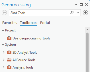
. - In the Geoprocessing pane, click the Toolboxes tab.
There are two separate headings for project and system toolboxes. Under the Project heading, the default toolbox appears, along with any other toolboxes you have added to the project. Under the System heading is an alphabetical list of toolboxes installed with ArcGIS Pro. Each toolbox
 contains a number of related tools, which may be further organized into toolsets
  .
.
- Under the System heading, browse to Analysis Tools > Pairwise Overlay.
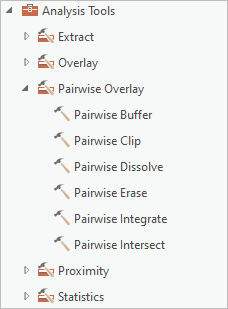
A toolbox or toolset may contain built-in tools
 , script tools
  , or model tools
  . The Pairwise Overlay toolset contains several built-in tools that provide better functionality and performance than classic overlay tools.
 - In the Pairwise Overlay toolset, click Pairwise Buffer.
The Pairwise Buffer tool opens in the Geoprocessing pane. Some of its parameters are blank; others have default values. Required parameters are marked with a red asterisk.
- Hover over the tool's Help button
 .
.A ScreenTip describes and illustrates the tool. The Pairwise Buffer tool creates distance zones around features. Buffers are often used to find features in one layer that include or exclude features in another layer. In this case, you will look for the presence of Nassella tussock within a specified distance of campgrounds.
Tip:
Click the Help button
 to open a geoprocessing tool's help topic.
Buffer the commercial campgrounds
Now you'll set the parameters and run the tool.
- On the Pairwise Buffer tool, click the Input Features drop-down arrow and click Commercial Campgrounds.
- In the Output Feature Class parameter, change the output dataset name from CommercialCamp_PairwiseBuffe to Campground_Buffers.
You can either highlight and replace the dataset name at the end of the path or delete the entire path and type the new feature class name. The full path will be restored automatically when the tool is run.
Tip:
Hover over the Output Feature Class parameter to see the path to the output dataset.
- In the Distance [value or field] box, type 1.5.
- Click the adjacent drop-down list of distance units and click Kilometers.
The tool will create a polygon feature class containing a buffer feature for each campground. The buffers will be circles of a 1.5-kilometer radius centered on the campgrounds. Your assumption is that campers are most likely to encounter Nassella tussock on walks and bike rides within this distance range.
- Hover over any tool parameter, such as Method or Dissolve Type.
An information icon
 appears next to the parameter.
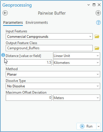
When you hover over the information icon, a ScreenTip describes the parameter and its settings. You'll accept the default values for the Method and Dissolve Type parameters.
- At the bottom of the Geoprocessing pane, click Run
 .
.Note:
The Run Modes
 option next to the Run
  button allows you to run tools on either the geoprocessing thread (the default) or the foreground thread. Using the geoprocessing thread allows you to work in ArcGIS Pro while the tool runs. Using the foreground thread improves processing time.
When the tool finishes running, a completion message appears at the bottom of the Geoprocessing pane.
- On the completion message, hover over View Details to see information about the process.
A new output feature class named Campground_Buffers is created in your default geodatabase, and a layer is added to the map. At the current map scale, the buffers are probably obscured by the campground symbols.
Note:
In the Geoprocessing pane, a warning icon
 appears next to the Output Feature Class parameter. This means that the feature class name has now been used. If you run the tool again without changing the name, you will overwrite existing data.
 - In the Contents pane, turn off the Commercial Campgrounds layer.
- Right-click the Campground_Buffers layer and click Zoom To Layer
 .
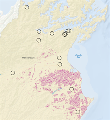
.The default buffer symbol is partially transparent. You'll change it to an outline to get a better look at Nassella tussock inside the buffers.
- In the Contents pane, click the symbol for the Campground_Buffers layer.

The Symbology pane appears and displays formatting options for polygon symbols.
- At the top of the Symbology pane, click the Gallery tab if necessary.
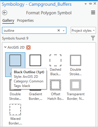
- Next to the search box, click the All styles drop-down arrow and click Project styles.
The Project styles setting includes the styles ArcGIS Pro adds to the project by default, as well as any other styles you add. The All styles setting includes all system styles installed with ArcGIS Pro. Choosing Project styles narrows the scope of symbol searches.
- In the search box, type outline and press the Enter key.
In the ArcGIS 2D style, a number of symbols are found. You can hover over the symbols to get more information.
- Click the Black Outline (1pt) symbol to select it.
The symbols are updated on the map.
- In the Contents pane, right-click the Campground_Buffers layer name and click Attribute Table
 .
.In the Campground_Buffers table, the name and address attributes have been copied from the Commercial Campgrounds layer that was the input to the Pairwise Buffer tool. The BUFF_DIST field shows the buffer distance expressed in meters.
- Close the attribute table.
- On the ribbon, click the Map tab. Zoom in and examine some buffers to see whether they contain Nassella tussock.
- When you're finished, in the Navigate group, click Bookmarks
 and click Campgrounds.
- On the Quick Access Toolbar, click Save Project
 .
.
Select buffers containing Nassella tussock
A visual inspection is helpful, but analysis is a more reliable way to identify the buffers that contain Nassella tussock. You'll use the Select By Location tool  to find features in one layer (Campground_Buffers) that have area in common with features in another layer (Nassella Tussock Range).
- In the Contents pane, click the Campground_Buffers layer to select it if necessary.
- On the ribbon, on the Map tab, in the Selection group, click Select By Location
 .
.The Select By Location window appears.
Note:
For convenience, some geoprocessing tools open in a floating window. These tools can also be opened in the Geoprocessing pane.
A key parameter for this tool is the spatial relationship to be evaluated. Depending on the situation, you may want to know whether features intersect, contain, touch, or lie within a certain distance of other features.
In this situation, containment might seem to be the right relationship because you want to find campground buffers that contain Nassella tussock. However, this choice is too restrictive. Imagine a patch of Nassella tussock that lies partly inside and partly outside a buffer. This patch is relevant to your analysis, but the buffer does not contain it; it only intersects it. On the other hand, if a patch lies entirely inside a buffer, the buffer both contains and intersects it. Therefore, you should use the intersect relationship.
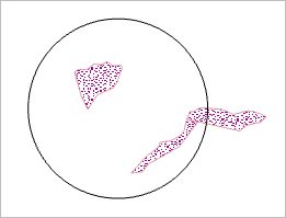
This buffer contains only one of the two features but intersects both. Intersection includes partial and complete overlap. Tip:
See Select By Location graphic examples for illustrations of how spatial relationships are defined with respect to points, lines, and polygons.
- On the Select By Location tool, confirm that the Input Features parameter defaults to Campground_Buffers and that the Relationship parameter is set to Intersect.
- Click the Selecting Features drop-down arrow and click Nassella Tussock Range.
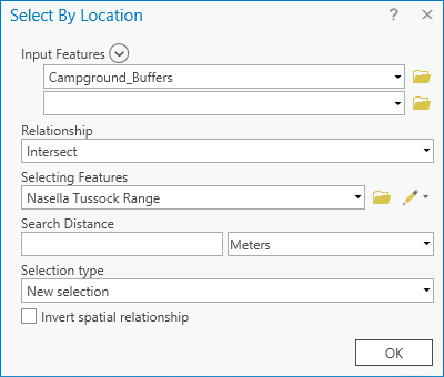
The features in the input feature layer are the ones that will be selected. You want to see which campground buffers are intersected by patches of grass, not which patches of grass are intersected by campground buffers.
There is no output feature class parameter because the Select By Location tool does not create a new dataset—it makes a selection on the input feature layer.
- Click OK.
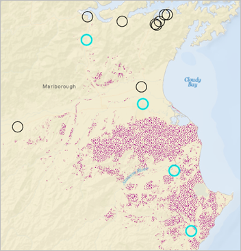
Four buffers are selected on the map. The number is confirmed by the message at the bottom of the map view.
Two of the selected buffers are in areas where Nassella tussock is prevalent and two are not. This raises the question of whether the four selected buffers have a geographic relationship that sets them apart from the others.
- In the Contents pane, turn on the Roads layer and expand it.
The four selected buffers are linked by principal highways. This suggests that the road network facilitates the spread of Nassella tussock. On the other hand, many unselected buffers are also linked by highways.
It would be useful to know which campgrounds are visited most often and whether vacationers typically visit multiple campgrounds, but these questions are beyond the scope of this tutorial.
- Turn off the Roads layer and turn on the Populated Places layer.
Three of the four selected buffers intersect populated places. At the same time, many populated places have no Nassella tussock near them. While this brief investigation was inconclusive, spatial selections allow you to discover patterns in your data and stimulate further analysis.
- Turn off the Populated Places layer.
- On the Quick Access Toolbar, click Save Project
 .
.
Quantify Nassella tussock within buffers
Finally, you want to know how much Nassella tussock lies within the selected buffers. This information can be shared with campgrounds and may help prioritize treatment. The measurements can also serve as a baseline for comparison in coming years.
You'll open the Summarize Within tool from the Analysis gallery. The Analysis gallery is a convenient place to access frequently used analysis tools.
- On the ribbon, click the Analysis tab.
- In the Tools group, expand the Analysis gallery.

Note:
Depending on the size of your ArcGIS Pro window, the Analysis gallery may appear as a button
 on the ribbon.
 - In the Analysis gallery, under Summarize Data, hover over the Summarize Within tool
 and read its description.
One of the functions of this tool is to calculate how much area of the polygons in one layer lies within the polygons of another layer. This is what you want to do.
- Click Summarize Within to open the tool in the Geoprocessing pane.
- Click the Input Polygons drop-down arrow and click Campground_Buffers.
When there is a selection on the input layer, geoprocessing tools work only on the selected features by default. In this case, only the four selected campground buffers will be processed and written to the output feature class.
Note:
You can click the Use the selected records toggle button to process all the features in the layer instead.
- Click the Input Summary Features drop-down arrow and click Nassella Tussock Range.
- For Output Feature Class, change the name to Tussock_Within_Buffers.
Like the Pairwise Buffer tool, the Summarize Within tool creates a feature class. The output features will have the same shapes as the input features. The only difference will be in the attribute table.
- Click the Shape Unit drop-down arrow and click Hectares.
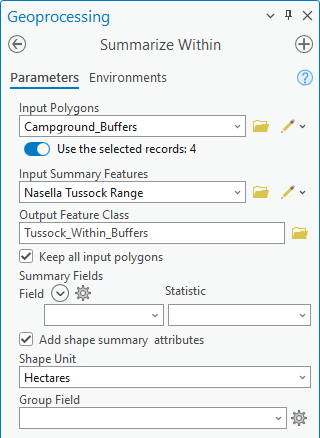
A hectare is a metric unit of area equal to 10,000 square meters or roughly two and a half acres.
- Click Run
 .
.When the tool completes, the Tussock_Within_Buffers feature class is created in the default geodatabase and a layer is added to the map.
- On the ribbon, click the Map tab. In the Selection group, click Clear
 .
. - In the Contents pane, turn off the Campground_Buffers layer.
The Tussock_Within_Buffers layer has four features, corresponding to the four selected campground buffers.
- In the Contents pane, right-click the Tussock_Within_Buffers layer and click Attribute Table
 .
. - In the table, right-click the BUFF_DIST field heading and click Hide Field
 . Hide the following fields as well:
- ORIG_FID
- Shape_Length
- Shape_Area
- Count of Polygons

The Summarized Area in HECTARES field contains the analysis results. (Remember that the Nassella Tussock Range layer represents areas within which the plant has been found, not the actual plant density.)
Tip:
To display hidden fields, click the Menu button
 on the table view and click Show All Fields.
 - Close the table.
- On the Quick Access Toolbar, click Save Project
 .
.
Visualize analysis results
You'll create a chart to visualize the analysis results.
- In the Contents pane, right-click the Tussock_Within_Buffers layer. Click Create Chart
 and click Bar Chart
  .
.The Chart Properties pane appears. A chart view appears as well. The view is empty until you configure the Chart Properties pane.
- At the top of the Chart Properties pane, confirm that the Data tab is selected. Click the Category or Date drop-down arrow and click Name.
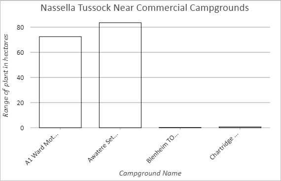
In the chart view, the campground names appear on the chart's x-axis. At the moment, the chart displays the count of names per campground (which is 1). You must choose the numeric field to chart and change the aggregation setting.
- In the Chart Properties pane, under Numeric field(s), click Select and check the Summarized area in HECTARES check box. Click Apply.
- Under Aggregation, click the drop-down arrow and click <none>.
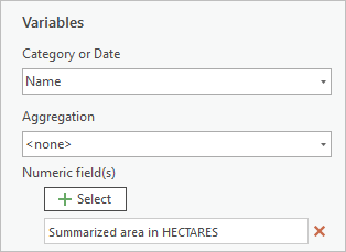
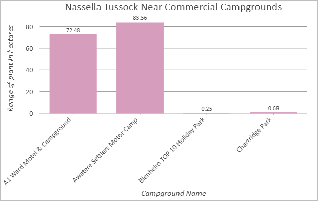
The chart's y-axis and data bars update to show the area covered by Nassella tussock around each campground.
Note:
Aggregation is only necessary when values in the category you are charting are represented by multiple records in the layer attribute table. In this case, each campground name corresponds to a single record in the table and aggregation is unnecessary. Learn more about aggregating category values.
- At the bottom of the pane, under Data Labels, check the Label bars check box.
The bars are labeled with their exact values, but you don't need to show so many decimal places. You will change this later when you format the axes.
- At the top of the Chart Properties pane, click the General tab. (If the pane is too narrow to display the tab, click More
 and click General in the drop-down list.)
 - In the Chart title box, replace the current title with Nassella Tussock Near Commercial Campgrounds and press the Enter key.
The title is updated on the chart.
- In the X axis title box, replace the current title with Campground Name and press the Enter key.
- In the Y axis title box, replace the current title with Range of plant in hectares and press the Enter key.
The campground names may display horizontally or diagonally depending on the size of your ArcGIS Pro window. You'll display them diagonally to make sure the complete names can be shown.
- Click the Axes tab. Under the X-axis heading, click the Label orientation drop-down arrow and click Diagonal.
- Under X-axis, change the Label character limit setting to 30 and press the Enter key.
The full name of each campground is displayed.
- Right-click the view tab of the chart and click Float.
The chart floats freely over the ArcGIS Pro window.
- Resize the chart by dragging any side or corner of the view.
- In the Chart Properties pane, on the Axes tab, under Number format, click Determine display formatting for numeric field types
 .
. - In the window that appears, click the Category drop-down arrow and click Numeric. Under Rounding, change the number of decimal places to 2.
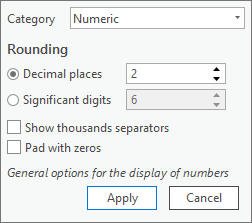
- Click Apply to update the bar labels on the chart.
By default, the data bar symbology matches the Tussock_Within_Buffers layer. While the outline symbol is useful on the map, it doesn't look good on the chart.
- In the Chart Properties pane, click the Series tab. In the table of fields, in the Symbol column, click the symbol to open the color palette.

- On the palette, click a color that you like.
The color of the data bars is updated on the chart.
- Close the chart view.
Tip:
To access the chart later, in the Contents pane, expand the Tussock_Within_Buffers layer. Under Charts, right-click the chart and click Open
 .
. - On the Quick Access Toolbar, click Save Project
 .
.
View geoprocessing history
ArcGIS Pro saves a record of the geoprocessing tools you use in a project. This geoprocessing history shows the order in which tools were run and saves the tool parameter settings. The geoprocessing history can help you retrace your steps, run tools with different settings to explore alternative outcomes, and modify the workflow. You can also use the history to help build a geoprocessing model or to create a geoprocessing package of tools and data to share with others.
- On the ribbon, click the Analysis tab. In the Geoprocessing group, click History
 .
.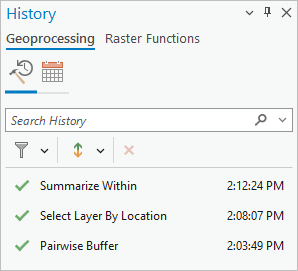
The History pane appears. On the Geoprocessing tab, on the Tool History tab
 , the geoprocessing tools you have run are listed. The green check marks show that the tools ran successfully.
In this analysis, you only used geoprocessing tools. If you had run any raster functions, you could see those history items on the Raster Functions tab.
- In the History pane, right-click the Pairwise Buffer tool and click View Details.
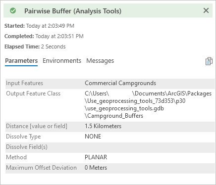
A window shows the parameter settings, environment settings, and other information. Error or warning messages associated with the tool, if any, also appear here. (The same information can be viewed on a tool's completion message in the Geoprocessing pane.)
- Close the message window.
You can also right-click the tool to open it, run it, add it to a geoprocessing model, or save it as a Python script.
The same workflow can often be accomplished in more than one way. For example, you could have skipped using the Select By Location tool and run the Summarize Within tool immediately on the campground buffers. In that case, your output feature class would have had 14 records instead of four. Ten records would have had values of 0 in the Summarized area in HECTARES field. However, an advantage of using the Select By Location tool is that it provides visual feedback that can reveal spatial patterns and suggest new directions for your analysis.
To see how the workflow in this tutorial can be modeled and run as a geoprocessing tool, try the Make a geoprocessing model tutorial.
