Understand ground classification

Ground classification is a fundamental processing step for aerial lidar. It unlocks much of the potential of the data, particularly for the creation of useful derivatives. DEMs, for example, are a common product made from aerial lidar, and ground classification is a required part of that process.

Other things people want to identify in lidar, such as buildings and vegetation, require ground classification to be performed first. This is because an inherent part of their classification process involves an assessment of how high a point is above the ground.

It is recommended that ground classification be performed by a professional and to have the data, along with any classifications applied, be examined by independent consultants to ensure it meets requirements. Requirements vary by project, though they often involve comparing ground classified heights to control point heights, and a review of hillshade derivatives from the ground classified lidar. The information in this topic describes how ground classification is performed using ArcGIS Pro.

Prerequisites and recommendations

Ground classification on point clouds is performed most commonly on aerial lidar. This is how the best, most consistent, view of the ground can be obtained. Photogrammetrically derived point clouds can also be used, although they are not as reliable as lidar for obtaining ground observations in vegetated areas.

Ground-based collection platforms, both stationary and mobile, can be problematic. Ground is often not captured reliably, as there are often shadows cast by objects on the ground. Additionally, the point density can vary, with many areas being oversampled or undersampled. Portions of scans in near proximity to the sensor may be appropriate. For example, the ground in immediate proximity to scans collected from a car or train, such as the road pavement or the railbed, can be captured in high quality. However, quality decreases as distance from the scanner increases or if there are many objects blocking the scanner’s view of the ground.

Point clouds of any type must be georeferenced and calibrated before ground classification. The data provider is typically responsible for this.

Overlap classification is also recommended so that the point density of the data considered for ground, and for other classifiers, is relatively consistent.

The data must be in a projected coordinate system. If the data is in decimal degrees, you can use the Extract LAS tool to project the data by setting an appropriate output coordinate system in the tool environment.

The data should be tiled. This involves partitioning it into nonoverlapping rectangular areas, which can be done using the Tile LAS tool. It is recommended that individual tiles of LAS format data not exceed 1 GB.

It’s recommended that the LAS data have statistics generated for them. Statistics creates a spatial index, which improves classification performance. The LAS dataset properties dialog box, and several LAS-related geoprocessing tools (Create LAS Dataset and LAS Dataset Statistics) can generate statistics.

If the data is being rewritten for any reason, for example, to project or to tile, it is recommended that you rearrange the point order when creating the files. This places points in a LAS file that are spatially close to one another, in terms of physical record sequence in the file, which improves the performance of spatial queries.

Perform ground classification

The Classify LAS Ground tool is used to automatically identify and classify ground points in lidar and photogrammetric point clouds. Once ground is classified, you can use the LAS Dataset To Raster tool to create a DEM, or classify the data further with other tools that rely on ground such as Classify LAS Building and Classify LAS By Height.

All of the points in a lidar point cloud.

Only the ground points in a lidar point cloud.

Only class 0 and class 4 1 points are considered for ground. Any existing class 2 ground 4 can be kept or removed (in other words, reset to class 1 and reconsidered for ground by the classifier) depending on the settings. There are also options for handling noise. By default, noise is left alone. All other existing classes are left unchanged.

Limitations

Classification of lidar is imperfect. With only the point information to work with, there isn't always a definitive right or wrong answer with some points. Consequently, there are multiple potential ground surfaces.

Try to use the best options to minimize error and reduce the amount of manual classification cleanup needed. Doing this successfully involves knowing the characteristics of both the data and the terrain in the study area.

Lidar-derived points generally yield better results than photogrammetrically derived points. This is due, in part, to the geometric characteristics of the points. Photogrammetric points generally don't capture the distinct transition where ground meets building, car, or vegetation as sharply as lidar. Also, photogrammetric techniques can't see to ground through vegetation the way lidar can.

Small areas collected by drones, such as a single building, often have a small amount of ground captured around the perimeter of the building. The ground classifier is less likely to find ground in these situations because there's little information to classify.

The pavement of overpasses and bridges tends to be misclassified as ground because roads leading to them are considered ground. Because there isn't a sharp break in slope as the road turns into an overpass or bridge, the classifier misclassifies, or expands, ground to go across.

Water is often misclassified as ground. This is because, from a geometric perspective as defined by the points, there's little difference between ground and water. Misclassified water should be corrected using polygon features that represent water bodies. Use these with the Set LAS Class Codes Using Features tool.

Clusters of low noise may be misclassified as ground because the classifier identifies them as potentially valid ground features, such as pits.

Interior scans of buildings, tunnels, or mine shafts are inappropriate for use with the Classify LAS Ground tool.

Use the Classify LAS Ground tool

While the Classify LAS Ground tool produces good results most of the time with the default parameters, you can use the various parameters to maximize quality and minimize error. The table below describes the parameters.

Ground Detection Method

This parameter includes three options: Standard Classification, Conservative Classification, and Aggressive Classification. These correlate with the amount of surface roughness and discontinuities that are accepted as ground. The Conservative option allows the least amount of roughness, while the Aggressive option allows the most. It is recommended that you use either Conservative or Standard, and reserve Aggressive for rugged terrain typically found in mountainous areas. Conservative is less likely to include nonground features but may miss valid ground in more rugged areas. Standard represents a good balance between the Conservative and Aggressive options when you have mixed terrain. The Conservative option is good for DEM generation because it reduces the chance of misclassifying low objects as ground. The Standard option is good for balancing omission error and commission error.

Detection Algorithm

This parameter includes two options: Latest and First Generation. The default is Latest. This option uses the newest generation classifier and is recommended. The First Generation option can be used, for example, to replicate or match results obtained using earlier software. In some cases, the First Generation option may have a more desirable result, but this is not typical.

Reuse existing ground

This optional parameter is either checked or unchecked. It's useful when at least some ground points have already been classified. Checking this parameter will keep the existing ground in place and add more to it. It's typically used when improving on an initial classification that missed some ground. This workflow is discussed in more detail below in the Fix problem areas section. When this parameter is unchecked, existing ground will be reclassified to class 1 and ground classification is redone from scratch. The default is unchecked.

DEM Resolution

Use this parameter when the cell size of the DEM you want to derive from the ground points is significantly coarser than the average point spacing of the input point cloud, and you want to reduce ground classification processing time. It's also a way to make thinned ground points that may have other uses. When using this parameter, a subset of ground points sufficient to make a DEM of the target resolution is classified. Since a smaller number of ground points are classified, the tool runs faster. The drawback is if you need higher-resolution ground in the future, you must rerun the classifier. This parameter requires the cell size provided to be greater or equal to 0.3 meters and that it be larger than 1.5 times the nominal point spacing of the point cloud.

Classify low-noise points

When checked, this parameter classifies points below ground as class 7 noise. If you provide a Minimum Depth Below Ground parameter value, only points deeper than that threshold will be classified as noise. The default threshold is 0, so any points below ground, regardless of depth, will be treated as noise. Checking the Classify low-noise points parameter is recommended because these points are unlikely to be interpreted, or classified, as a different class. It's more helpful to have them assigned to the noise class, rather than left in class 0 or 1, if they can't possibly be anything else. Not all below ground points, or more correctly, what appears to you as below ground, will be classified as low noise. This mostly occurs with clusters of points because the classifier identifies them as potentially valid features, such as mines or pits.

Preserve existing low noise

When checked, this parameter preserves any existing low noise points, with the intention of adding more low noise. The default is off, where any existing low noise will first be reset to class 1, and then get evaluated from scratch.

Classify high-noise points

When checked, this parameter classifies points above ground, by the Minimum Height Above Ground parameter value provided, as class 18 high noise. It's intended to find noise associated with clouds, haze, and high-flying birds. Use a threshold that's higher than trees, buildings, and other tall infrastructure so they are not classified as noise. Note: If you only have a few valid tall features in the landscape, but a lot of high noise within the height range of those features, it can be advantageous to provide a height threshold that will result in the misclassification of the tall features. This is because it can be easier to fix those few problem spots manually than to fix all the missed noise that will result from a higher height threshold.

Preserve existing high noise

When checked, this parameter preserves existing high noise points, with the intention of adding more high noise. The default is off, where any existing high noise will first be reset to class 1, and then get evaluated from scratch.

Review results

No classification is perfect. The results should be reviewed and cleaned up manually as needed. There are two types of problems: points that should have been classified as ground that weren’t (errors of omission), and points that were classified as ground that shouldn’t have been (errors of commission).

You can try to find errors by reviewing the statistics. For example, by examining ground point height ranges in the Statistics pane of the LAS Dataset Properties dialog box from the Catalog pane, to see whether they fall within expected ranges. You can also test heights against other height sources, such as survey data or pre-existing DEMs, and look for significant differences.

One of the most common technique is to derive a hillshade raster from a DEM that was created from the ground classified points, and have someone visually review the hillshade for anomalies. The purpose of this is to look for unnatural-looking landforms. These include unusual peaks and pits, but what is more likely are missing, or truncated, ridges in rugged terrain.

Fix problem areas

Isolated problem spots, like a pit that should be low noise, should is probably best fixed manually. To do this, build a pyramid for the LAS dataset and view the point cloud by class code in a local 3D view. Ensure that the spatial reference for the view is the same as the point cloud. The LAS dataset layer ribbon has a Classification tab that includes tools for selecting and reclassing specified points.

Sharp ridges can be lost in rugged terrain when the classification method is set to Conservative or Standard. While you can use the Aggressive method to avoid this, its use is not recommended unless the entire area is rugged. In the more common scenario of mixed terrain, it's better to use either the Conservative or Standard methods to obtain quality results in the less rugged areas. The trade-off is the classifier can be too restrictive in rugged areas. It identifies sharp changes in slope as unlikely to be ground, and can miss ridgelines, especially in heavily forested areas that have fewer ground hits.

To overcome problem ridges, a derived hillshade is first made from the initial ground classified points. It's used to identify problem locations. The operator digitizes polygons around problem areas. The polygons don't need to be precise. The ground classifier is then rerun, using a less restrictive method than the initial run. If the Conservative classification was used, try Standard. If Standard was used, try Aggressive. Also, check the Reuse existing ground parameter to retain the existing ground, and have the polygon feature class containing problem polygons used as the processing extent. The polygon selection is honored, so you can pick specific areas to process and iterate over.

This will automate a more aggressive classification just for those problem areas while leaving the other areas, classified more conservatively, alone. Another review should be made for each problem area after this re-running of the classifier.

Edit ground seed points manually

For an area that remains problematic, even after using the Aggressive classification, you can manually classify a few ground seed points along the top of the ridge, select the corresponding problem polygon, and rerun the tool using the same parameters: aggressive detection, reuse of ground checked, and the selected problem polygon for a processing extent. The seed points will help the classifier find more points along and around the ridge.

To edit ground seed points manually, complete the following steps:

1. Locate the problem spot in a 3D view.
   1. Add the DEM as the scene ground model.
   2. Drape the hillshade and problem polygons (symbolized with outlines but no fill) on the ground.
   3. Navigate to a problem area.
2. Orient the view so you are looking top down on the data.
3. Select the LAS dataset layer in the Contents pane, but leave the points turned off.

   Selecting the LAS dataset layer enables the LAS Classification tab on the ribbon, along with the Profile tool, but leaving the points off allows you to see where to draw a profile.

4. Once the profile has been drawn and the profile view appears, turn off the draped hillshade and polygons, and turn the points on.
5. Rotate the view so you're looking along the ridge instead of a side view of it.
6. Optionally, turn off Visible Points so that multiple ground points along the ridgetop, near and far, can be selected at one time.
7. After manually classifying some ground seed points, rerun the classifier using the corresponding problem area polygon as the processing extent.

The orientation of the profile view has been rotated so the camera is at one end of the ridge looking along it. This makes it easier to see the crown of the ridge and select the ground points.

The following images show different ways to visualize a ground surface in 2D for identifying problem areas and assessing the fixes made for them:

The 2D map views are based on the LAS dataset drawn as a triangulated surface symbolized by a combination of slope and hillshade.

Note:

The more pronounced green in the problem area is evident before the repair. Green represents lower slope and is indicative of what happens when the top of a ridge hasn't been captured properly.

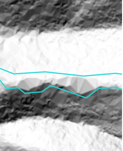
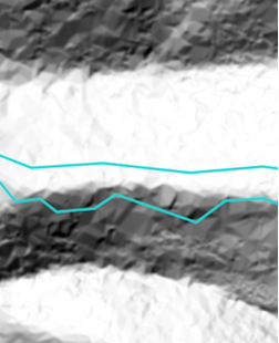
The images above are similar to the previous example except for the use of hillshade alone, without being colored by slope. Visual review of hillshades is a commonly used approach to identify problems with ground classification.