Image Classification Wizard

Available with Image Analyst license.

Available with Spatial Analyst license.

Image classification is the process of extracting information classes, such as land-cover categories, from multiband remote sensing imagery. The workflow involves multiple steps to progress from preprocessing to segmentation, training sample selection, training, classifying, and assessing accuracy. Each step may be iterative, and the process requires in-depth knowledge of the input imagery, classification schema, classification methods, expected results, and acceptable accuracy.

Classification Wizard

The Classification Wizard guides users through the entire classification workflow from start to finish. The Classification Wizard provides a guided workflow that is composed of best practices and a simplified user experience, so you can perform image classification without missing a step. Experienced users can use individual tools available in the Classification Tools drop-down list in the Image Classification group. These tools are the same ones included with the Classification Wizard.

The Classification Wizard is found in the Image Classification group on the Imagery tab. Select the raster dataset to classify in the Contents pane to display the Imagery tab, and be sure you are working in a 2D map. The Classification Wizard is disabled if the active map is a 3D scene, or if the highlighted image is not a multiband image.

Configure

Click the Classification Wizard button on the Imagery tab to open and dock the wizard. The first page is the Configure page, where you set up your classification project. The parameters set here determine the steps and functionality available in the subsequent wizard pages.

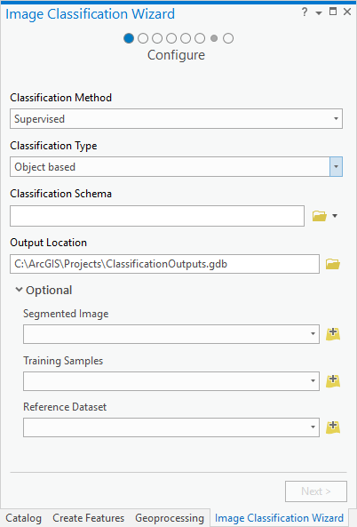
Classification Method

There are two options for the method you will use to classify your imagery.

Option name	Description
Unsupervised	The outcome of the classification is determined without training samples. Pixels or segments are statistically assigned to a class based on the ISO Cluster classifier. Pixels are grouped into classes based on spectral and spatial characteristics. You provide the number of classes to compute, and the classes are identified and merged once the classification is complete.
Supervised	The outcome of the classification depends on the training samples provided. Training samples are representative sites for all the classes you want to classify in your image. These sites are stored as a point or polygon feature class with corresponding class names for each feature, and they are created or selected based on user knowledge of the source data and expected results. All other pixels in the image are classified using the characteristics of the training samples. This is the default option.

Classification Type

There are two options for the type of classification to use for both supervised and unsupervised classification.

Option name	Description
Pixel based	Classification is performed on a per-pixel basis, where the spectral characteristics of the individual pixel determines the class to which it is assigned. Characteristics of neighboring pixels are not considered in the pixel-based approach. This is considered the more traditional classification method, and can result in a speckled effect in the classified image.
Object based	Classification is performed on localized neighborhoods of pixels, grouped together with a process called segmentation. Segmentation takes into account both color and shape characteristics when grouping pixels into objects. The objects resulting from segmentation more closely resemble real-world features and produce cleaner classification results. This is the default option.

Classification Schema

A classification schema determines the number and types of classes to use for supervised classification. Schemas can be hierarchical, meaning there can be classes with subclasses. For example, you can specify a class of Forest with subclasses for Evergreen and Deciduous forests. A schema is saved in an Esri classification schema file (.ecs), which uses JSON syntax. You can choose from the following options to specify the classification schema:

• Browse to an existing schema.
• Generate a schema from an existing feature class representing training samples. Choose this if you plan to reference an existing training samples dataset.
• Generate a schema from an existing raster class map.
• Use the default schema from the National Land Cover Dataset for North America. If you want to create a custom schema, choose this option and modify it on the Training Sample Manager page.

Output Location

This is the workspace or directory that stores all of the outputs created in the Classification Wizard, including training data, segmented images, custom schemas, accuracy assessment information, and classification results.

Note:

All intermediate files created using the Classification Wizard are stored in the user temp directory. This is typically C:\Windows\Temp, but it may be different based on the operating system and access permissions.

Segmented Image

This is only an option if you selected Object based classification for Classification Type. If you have already created a segmented image, you can reference the existing dataset. Otherwise, you will create a segmented image as a step on the next page.

Note:

If the segmented raster has not been created previously, it will be created before training the classifier. This is a computer-intensive operation, and it may take a significant amount of time to create the segmented raster dataset. For large datasets, it is highly recommended that you create the segmented raster beforehand and specify it as an input when you configure your classification project.

Training Samples

This is only an option if you selected Supervised for Classification Method. You can create training samples using the Training Samples Manager pane in the Classification Tools drop-down list, or you can provide an existing training samples file. This can be either a shapefile or a feature class that contains your training samples, and it must correspond with the classification schema. The following field names are required in the training sample file:

• classname—A text field indicating the name of the class category
• classvalue—A long integer field containing the integer value for each class category

Note:

Training samples created in ArcGIS Desktop using the Image Classification toolbar are supported.

Reference Dataset

If you want to assess the accuracy of classified results, you need to provide a reference dataset. Reference data consists of features with a known location and class value, and it can be collected using a field survey, an existing class map or raster land base, or with higher-resolution imagery. The results of your image classification will be compared with your reference data for accuracy assessment. The classes in your reference dataset need to match your classification schema.

Reference data can be in one of the following formats:

• A raster dataset that is a classified image.
• A polygon feature class or a shapefile. The format of the feature class attribute table needs to match the training samples. To ensure this, you can create the reference dataset using the Training Samples Manager tools.
• A point feature class or a shapefile. The format needs to match the output of the Create Accuracy Assessment tool. If you are using an existing file and want to convert it to the appropriate format, use the Create Accuracy Assessment Points geoprocessing tool.

Segmentation

This page is only available if you selected Object based as your Classification Type, and you did not specify an existing segmentation raster dataset on the Configure page. Segmentation is a key component of the Object based classification workflow. This process groups neighboring pixels together that are similar in color and have certain shape characteristics.

There are three parameters that control how your imagery is segmented into objects:

• Spectral Detail—Set the level of importance given to the spectral differences of features in your imagery.

  Valid values range from 1.0 to 20.0. A higher value is appropriate when you want a more detailed classification, where features that have somewhat similar spectral characteristics are to be classified into different classes. For example, with higher spectral detail values for a forested scene, you can have greater discrimination between the different tree species.

  Smaller values result in more smoothing of image detail. For example, if you are interested in classifying building roofs without any detail about the equipment on the roof, use a lower Spectral Detail value.

• Spatial Detail—Set the level of importance given to the proximity between features in your imagery. Valid values range from 1 to 20. A higher value is appropriate for a scene where your features of interest are small and clustered together. Smaller values create spatially smoother outputs. For example, in an urban scene, you can classify impervious surfaces using a smaller spatial detail value, or you can classify buildings and roads as separate classes using a higher Spatial Detail value.
• Minimum segment size in pixels—Merge segments smaller than this size with their best-fitting neighbor segment. This value is related to the minimum mapping unit of your project.

You can use the Show Segmented Boundaries Only option if you want to display the segments as polygons overlaid on your imagery.

Use the Swipe tool in the Effects group on the Raster Layer or Mosaic Layer tab to compare your segmented image with the source image. Dynamically rerun the segmentation by changing the parameters, and examine the results by panning and zooming the map. When you are satisfied with your segmented image, click Next.

Note:

The preview is based on raster functions that process pixels currently on display and resampled to display resolution. This may cause a slight difference between the preview and the actual persisted result for regional operations.

Training Samples Manager tools

This page is only available if you select Supervised for Classification Method.

When the page opens, you can see the schema management section at the top, where the schema you selected on the Configure page is automatically loaded. You can create new classes here or remove existing classes to customize your schema. To create a new parent class at the highest level, select the name of your schema and click the Add New Class button. To create a subclass, select the parent class and click Add New Class. The subclass will be organized into the parent class. Right-click any of the classes to edit the class properties.

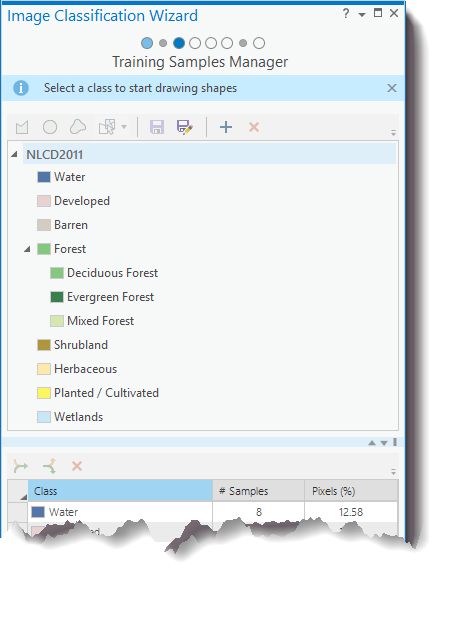
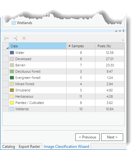
The bottom section of the page shows you all of the training samples for each class. You can select representative sites, or training samples, for each land-cover class in the image. A training sample has location information (polygon) and an associated land-cover class. The image classification algorithm uses the training samples, saved as a feature class, to identify the land-cover classes in the entire image. If you provided a training samples dataset on the Configure page, you will see your training samples listed here.

You can view and manage training samples by adding, grouping, or removing them. You can remove training samples individually, or you can group them together by selecting them and clicking the Delete button. When you select a training sample, it is selected on the map. Double-click a training sample in the table to zoom to it in the map.

To create training samples, complete the following steps:

1. Select the class that you want to collect training samples for in the schema manager.
2. Select one of the sketch tools or use the segment picker to begin collecting your training samples.
   1. To use the Segment Picker tool, the segmented image must be in the Contents pane. If you have more than one segmented layer in the Contents pane, use the drop-down list to select the segmented layer that you want to collect training samples from.
   2. Click the map to add the segment as a training sample.

   The individual training samples representing a class are listed in the Training Samples Manager.

3. You can organize them by selecting multiple training samples and combining them into one class heading by clicking the Collapse button .

Note:

The training samples table lists the number of samples defining each class. If you used the segment picker tool to collect your training samples, the number of samples is the number of segments you selected to define the class. This is important to remember when you use a statistical classifier such as Maximum Likelihood, because the number of segments represents the total number of samples. For example, if eight segments were collected as training samples for a class, it may not be a statistically significant number of samples for reliable classification. However, if you collected the same training samples as pixels, your training sample may be represented by hundreds or thousands of pixels, which is a statistically significant number of samples.

The training samples table lists the percentage of pixels representing a class compared to the total number of pixels representing all classes. This percentage is important when using a statistical classifier such as Maximum Likelihood. The number and percentage of training samples is less important when using the nonparametric machine learning classifiers, such as Random Trees and Support Vector Machine.

Train

Select one of the classification methods described in the following table:

Classifier	Description
ISO Cluster	The ISO Cluster classifier performs an unsupervised classification using the K-means method. This classifier can process very large segmented images, whose attribute table can become large. Also, the tool can accept a segmented RGB raster from a third-party application. The tool works on standard Esri-supported raster files, as well as segmented raster datasets. If you selected Unsupervised for Classification Method on the Configure page, this is the only classifier available.
K-Nearest Neighbor	The K-Nearest Neighbor classifier performs a K-nearest neighbor classification, which classifies a pixel by a plurality vote of its neighbors. The training process assigns the training samples to their respective classes. K is the defined number of neighbors used in voting.
Maximum Likelihood	The Maximum Likelihood classifier is a traditional parametric technique for image classification. For reliable results, each class should be represented by a statistically significant number of training samples with a normal distribution, and the relative number of training samples representing each class should be similar.
Random Trees	The Random Trees classifier is an advanced machine learning technique that is resistant to overfitting, and can work with segmented images and other ancillary raster datasets as well as multispectral imagery. For standard image inputs, the tool accepts multiple band imagery with any bit depth, and it will perform the Random Trees classification (sometimes called random forest classification) based on the input training sample file. If you chose Object based classification, you can select any or all of the segment attributes to be used in training the classifier.
Support Vector Machine	The Support Vector Machine classifier is an advanced machine learning classification method that is able to process a segmented raster input or a standard image. It is less susceptible to noise, correlated bands, and an unbalanced number or size of training sites within each class. The kernels use are nonlinear radial basis function (RBF), using a 2D grid with optimal parameter pairs (C, gamma). If you chose Object based classification, you can select any or all of the segment attributes to be used in training the classifier.

When you click Run, the classifier will be trained.

After it finishes running, you can visually verify the results with the source image using the Swipe tool on the Raster Layer or Mosaic Layer tab. You can compare the results using different settings or use different classifiers by clicking Previous and adjusting settings or by selecting a different classifier to run. You can then compare the different classification results using the Swipe tool or by clicking layers on and off in the Contents pane. Once you are satisfied with your classification results, click Next.

Classify

Click Run to save the results of the classification to the specified output directory or project database. Optionally, you can save the output class definition file (.ecd).

Assign Classes

This page only appears if you chose Unsupervised for Classification Method. A number of classes were created, depending on how many classes you specified, and using the pixel or segment characteristics of your source imagery. Now, you need to assign meaning to each class based on the classification schema you are using. The top of the Assign Classes page shows the list of classes in your schema, and at the bottom a table displays the classes that were generated.

1. Select a class from the schema list at the top of the page.
2. Click the Assign tool and select the classes on the class map that you want to assign to the schema class. As you are assigning classes, review the underlying imagery to verify that the New Class values make sense. Press the L key to change the transparency of the classified image. Inspect the table and confirm that it has updated the Old Class value with the class you have assigned it to. The class color is updated to reflect the schema.

   If you uncheck the class map in the Contents pane so that the source image is displayed, you can click features in the imagery, such as gray roofs or lawns, which will continue to reassign the corresponding classes in the class map.

Merge Classes

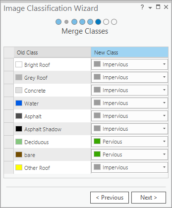
After performing a supervised classification, you can merge multiple classes into broader classes. The original class names are listed in the Old Class column of the Merge Classes page. If you want to change an entire class you can do that here, but you are limited to the parent classes in your schema. For example, you can change deciduous to forest, but you can't change deciduous to water on this page. To make those types of edits, or to change individual features, use the Reclassifier page.

Accuracy Assessment

The results of your image classification will be compared with the Reference Data you provided on the Configure page for accuracy assessment. The classification schema of the reference dataset must match that of the classified image.

Number of Random Points

The total number of random points that will be generated.

The actual number may exceed but never fall below this number, depending on the sampling strategy and number of classes. The default number of randomly generated points is 500.

Sampling Strategy

Specify a sampling method to use:

• Stratified Random—Create points that are randomly distributed within each class, and each class has a number of points proportional to its relative area. This method samples the image so that the number of sample points per class is proportional to the area per class in the image. The final accuracy assessment result is representative of the image. This is the default.
• Equalized Stratified Random—Create points that are randomly distributed within each class, and each class has the same number of points. This method assigns the same number of sample points to each class, regardless of how much area each class has in the image. The final accuracy assessment result is not representative of the image, but measures the accuracy by giving the same weight to each class. This is an alternative method to stratified random sampling for accuracy assessment.
• Random—Create points that are randomly distributed throughout the image. This method samples the points randomly over the image. There is no stratification involved, so the final accuracy assessment result is representative of the image; however, when a small number of sample points are used, some classes representing small areas may be missed or underrepresented.

Analyzing the diagonal

Accuracy is represented from 0 to 1, with 1 being 100 percent accuracy. The colors range from light to dark blue, with darker blue meaning higher accuracy. Values along the diagonal represent overall accuracy of class assignment.

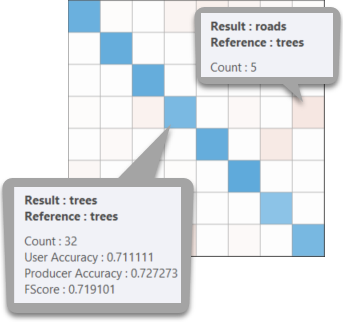
Analyzing off the diagonal

Unlike the diagonal, the cells that are off the diagonal show errors based on omission and commission. Errors of omission refer to pixels or segments that were left out from the correct class in the classified image, so the true class was omitted or diminished in the classification. Errors of commission refer to the incorrect classification of pixels into a class, falsely increasing the size of the class. An error of omission in one class is counted as an error of commission in another class.

If you want to examine the error matrix values, load and open the output confusion matrix saved in your project or output folder. This error report, in .dbf format, lists the user and producer error for each class and includes the kappa statistic agreement for the overall accuracy.

Once you decide that the accuracy of your image classification is acceptable for your purposes, you can move on to the final page of the Classification Wizard. If not, you may consider re-creating your training samples, adjusting the parameters or using a different classification, or testing with different reference data.

Reclassifier

After you classify an image, there can be small errors in the classification result. To address these errors, it is often easier to edit the final classified image rather than re-create training sites and perform each step in the classification again. The Reclassifier page allows you to make edits to individual features or objects in the classified image. This is a postprocessing step designed to account for errors in the classification process. All changes that you make are displayed in the Edits Log file, and you have the option to check on or off any of the edits you have made. As you reclassify the image to correct errors, review the underlying imagery to verify that the objects make sense. Press the L key to change the transparency of the classified image.

1. For Current Class and New Class, select classes for the reclassification.
2. Reclassify an object or class within a region.
   • Use the Reclassify an object tool to draw a circle on the classified image. The segment from which the circle originates will be changed to the new class.
   • Use the Reclassify within a region tool to draw a polygon on the classified image. The current class within this polygon will be changed to the new class.
3. Verify the edits you will keep or discard using the edits log, and name the final classified dataset that will be stored in the output location you set on the Configure page.