Available with Spatial Analyst license.
The path distance tools, Path Distance, Path Distance Allocation, and Path Distance Back Link, are used for distance analysis. Using these in conjunction with the Cost, Euclidean, Hydrologic, and other Spatial Analyst tools, many dispersion and movement processes can be effectively modeled. The next sections describe the basic theory behind the path distance tools and how to use them.
The basic rules of motion behind path distance
The path distance tools are similar to the cost distance tools in that both determine the minimum accumulative travel cost from a source to each cell location on a raster. However, path distance not only calculates the accumulative cost over a cost surface, it does so while compensating for the actual surface distance that must be traveled and for the horizontal and vertical factors influencing the total cost of moving from one location to another. The accumulated cost surface produced by these tools can be used in dispersion modeling, flow movement, and least-cost path analysis.
To make the most efficient use of path distance tools, you must understand some basic principles of dispersion and movement over a surface. To illustrate these basic principles, the amount of energy will be explored, or more explicitly, the amount of fuel needed to drive a car between two points while encountering various cost factors.
To drive a car on a flat road 50 miles from point A to point B will require x gallons of fuel.
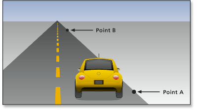
More fuel will be needed to drive the same car from point A to point B if it has to travel on a rough or bumpy surface, such as an unpaved road. The amount of fuel used in the second instance is calculated by the distance traveled over the friction, which is the friction factor (F), to compensate for the bumpiness of the surface, times the distance to travel divided by the miles per gallon the car gets on flat, smooth surfaces (D = Miles traveled / miles per gallon), resulting in the following formula:
F * D = fuel_used 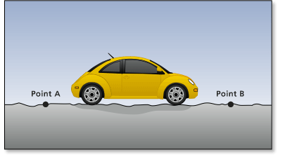
The above formula can also be used in the first example, but the friction factor was much lower than in the second example because the car traveled on a smooth surface.
If the route from point A to point B was uphill, the car would have to travel farther in actual distance than if the route were flat. (You can ignore for the moment the fact that additional fuel would be necessary to propel the car uphill.) The distance that would be traveled is referred to as the surface distance (SD).
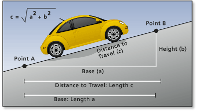
The surface distance extends the actual travel distance over the type of travel surface. Continuing the preceding example, the car now must travel on the bumpy surface for a longer distance. The surface distance (SD) increases the total cost of travel as a factor, not by simple addition. When considering surface distance (SD replaces D), the following formula is used:
F * SD = fuel_usedAnother group of elements that might influence a car's consumption of energy is the horizontal factors. These factors consider the easiest horizontal route to travel and how far from it the car is traveling. One horizontal factor in this example could be wind speed. If there is a strong wind behind the car, it will use less fuel to move from point A to B, regardless of the surface and actual travel distance.
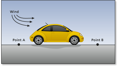
Including the horizontal factor (HF) in the total cost of travel results in the following formula:
F * SD * HF = fuel_usedThe horizontal factor related to wind speed must be adjusted to compensate for the amount of horizontal friction that will be encountered with regard to the relationship of direction of travel and wind direction. For example, if the wind is blowing behind the car at a 45-degree angle offset, the wind will be of some advantage to the car but not as much as if blowing directly behind it (a 0-degree offset).
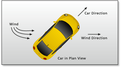
If the car is heading directly into the wind, the horizontal friction factor would be greatest.
The final factor that will affect the energy consumption of the car is the uphill or downhill slope that must be overcome during travel, which is called the vertical factor. In this example, if the car is going downhill, the total cost of travel will decrease; if it is going uphill, the total cost will increase.
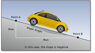
Incorporating the vertical factor (VF) into the previous formula results in the following formula:
F * SD * HF * VF = fuel_usedWhen modeling a source of dispersion or a moving object, a path distance tool will allow for control of the friction, surface distance, horizontal factor, and vertical factor. The example presented above is a simple one, but many of the elements affecting motion can be illustrated. Most movement is not as simple as a car traveling on a surface. For instance, it may be least costly for some types of phenomena when the vertical angle is great or when it deviates significantly from the specified horizontal direction of travel. Zero slope may be costly to overcome in another situation. Slope for the vertical factors may be air densities, concentration levels, or noise decibels rather than elevation. Path distance tools allow the control of the factors that influence dispersion, such as the ones listed here, allowing for customization of the analysis to meet the requirements of the phenomenon under consideration.
Outputs from path distance analysis
The different types of output from the path distance tools are described in the following sections.
Path distance output
The primary output from the Path Distance tool is the total accumulative cost distance raster. This raster stores the least cost accumulated distance for each cell, accounting for all the cost factors, that results from the least costly source cell. Since the cost distance is based on an iterative allocation, the lowest accumulative cost for each cell from a source is guaranteed. The accumulative values are based on the cost unit specified on the cost surface.
Path distance back link direction output
The Path Distance Back Link tool identifies, for each cell, which cell to move or flow into on its way back to the source from which it is least costly to reach.
The values in the output raster range from 0 through 8, which are codes that identify the direction to the next neighboring cell (the subsequent cell) when retracing (from the destination to the least costly source) the least accumulative cost path. The source cells are assigned 0 since they are already at the goal (the source).
If the path passes into the neighbor to the right, the output cell will be assigned the value 1. If the path is to the lower right direction, the value will be 2, directly south would be 3, and so on, continuing in a clockwise direction, as demonstrated in the following diagram:

Path distance allocation output
The Path Distance Allocation raster identifies, for each cell, the zone of the source that can reach the cell location with the least accumulated cost.
The output values are the same as the value of the input source, unless a value for Input Value Raster is specified, in which case the values in that input would be used.
Optional outputs
In addition to the specific output raster from each tool, each of the path distance tools can also optionally create other types of outputs. The Path Distance tool can create a back link raster, and the Path Distance Back Link tool a distance raster. The Path Distance Allocation tool can also create both the distance and back link rasters, which is useful if you want to create all the possible outputs with the execution of a single tool.
Inputs to path distance tools
A dataset of source locations is the required input to all path distance tools. Depending on the particular tool and options being used, other inputs can be specified to further control the analysis.
The source input
The source input identifies those locations from which a least accumulative cost distance is calculated to each non-source cell. It can be a feature dataset or a raster dataset, the same as you would use for the cost distance tools.
A source input can contain single or multiple zones. These zones may or may not be connected. The original values assigned to the source cells are retained. There is no limit to the number of source cells within the <source> raster.
The cost input
The input cost raster is also the same as what you would use in the cost distance tools. Each cell location is given a weight proportional to a relative cost incurred by the phenomenon being modeled when passing through a cell. The costs are usually based on inherent features in the location that are static prior to the movement of the feature or phenomenon. If modeling fire movement, for example, the cost features might include slope, aspect, age, type, moisture content, and canopy cover of the vegetation.
The cost units are based on any relative scale, not in geographic units. The units can be dollar cost or energy units expended; preference costs can be unitless. What is most important is that the values be in a relative scale. Adding the values associated with slope, aspect, and vegetation type will give meaningless results to fire movement. However, if each of these attributes is reclassed in relation to fire susceptibility, then added, the results will be a fire cost raster.
The cost values assigned to each cell are per unit distance measures for the cell.
By interpreting the costs stored at each cell as the cost-per-unit distance of travel through the cell, the analysis becomes resolution independent. Suppose there are two rasters, one at 50-meter resolution and the other at 100-meter resolution. Several adjoining cells in each raster are assigned five cost units to travel through each cell. The five cost units are applied to each unit of distance (the cost to move a meter in this case); therefore, it will cost 500 cost units to move 100 meters through the cells in either of the two rasters regardless of their resolution.
Example
If the cell size is expressed in meters, the cost assigned to the cell is the cost necessary to travel one meter within the cell. If the resolution is 50 meters, the total cost to travel will then depend on whether the travel is:
- Perpendicular through the cell (either horizontally or vertically), where it would be the cost assigned to the cell multiplied by the resolution (total_perpendicular_cost = cost * 50).
- Diagonally through the cell, where it would be the cost assigned to the cell multiplied by the cell resolution, multiplied by the diagonal factor of ≈1.414214, or √2, (total_diagonal_cost = 1.414214 *(cost * 50)).
The surface raster
An input surface raster can be used to determine the actual surface distance, as opposed to the planimetric ("straight-line") distance, traveled from one cell to the next. Elevation is usually the input surface raster.
The Pythagorean theorem is used to calculate the actual travel distance from cell a to cell b:
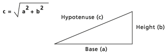
- If the cost is calculated to one of the four adjacent neighbors, the length of the base (a) is equal to the cell size (the distance from the center of one cell to the center of another).
- If the cost is determined to a diagonal cell, the base is derived from the cell size times ≈1.414214 (or, √2).
To determine the height (b) of the triangle, the height of the To cell on the surface raster is subtracted from the height of the From cell.
When the surface is not flat, the travel distance is greater. Greater distance means that more cost is incurred at the rate determined by the input cost raster and by the horizontal and vertical factors.
The cost of overcoming the angle of incline or decline (slope) is not necessarily calculated only from the surface raster. The costs associated with the slope angle are calculated from the input vertical factor raster and accompanying vertical cost factors. The raster used for the vertical factor raster can be the same as the raster used for the input surface raster.
More details on controlling path distance calculations
Defining a maximum distance threshold
Sometimes a threshold accumulative cost is reached beyond which you are interested. Such a threshold is controlled by the maximum distance parameter. Any location that exceeds the threshold will receive NoData on the output cost distance raster.
Using alternative values on the allocation output raster
If the values associated with the source cells on the input source raster are to be replaced by alternative values on the output allocation raster, a value raster can be input. The values defined for each source cell by the value raster will be assigned to all cells that are allocated to the source cell location in the cost allocation raster.
Variations on the elements
Many variations can be modeled with Path Distance by altering one or all input parameters. For instance, if there is no input surface raster to calculate surface distance, nor horizontal or vertical factor cost elements, Path Distance will perform the same calculations as the Cost Distance tool. When cost distance is calculated over a flat surface, there is no need for an input surface raster.
Sometimes one of the horizontal or vertical factor rasters may contain the same value for every cell location. For instance, when trying to model wind in a situation where the micro-topography is of no concern and the winds are prevailing from a single direction (such as southeast), every cell location on the horizontal raster can be set to 45 degrees.
Units for the input factors
Remember the following effects when determining the cost factors:
- Any positive or negative slope between cells increases the surface distance, thus increasing the cost.
- A horizontal or vertical factor of 1 does not affect the cost to move between cells. However, a factor less than 1 decreases the cost, and a factor greater than 1 increases it.
When determining the horizontal or vertical factor function to use (especially when altering it with modifiers) or when creating a custom factor graph, the initial cost units on the input cost raster and the effects of a factor on these units must be kept in mind.
How path distance is calculated
To learn more about how the outputs from the path distance tools are calculated, proceed to the following section: