Disponible con una licencia de Geostatistical Analyst.
You may want to remove a surface trend from your data and use kriging or cokriging on the detrended (residual) data. Consider the additive model:
Z(s) = µ(s) + ε(s),where µ(s) is some deterministic surface (the trend) and ε(s) is a spatially autocorrelated error.
Conceptually, the trend is fixed, which means that if you simulate data again and again, then the trend never changes. However, you do see fluctuations in the simulated surfaces due to the autocorrelated random errors. Usually, the trend changes gradually through space, while the random errors change more quickly. A meteorological example of a trend might be where you observe (and know theoretically) a temperature gradient with latitude. However, observations on any given day show local variations due to weather fronts, ground cover, cloud patterns, and so on, that are not so predictable, so the local variations are modeled as being autocorrelated.
Unfortunately, there is no magical way to decompose data uniquely into a trend and random errors. The following is offered to serve as a useful guide.
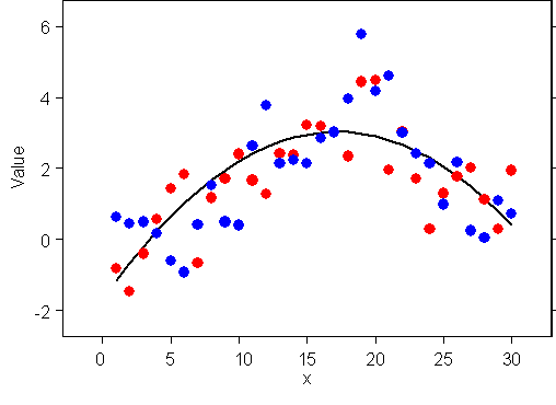
In the following detrending graph, data was simulated from two models. One was from the Ordinary Kriging model, where Z(s) = µ + ε(s) and the errors e(s) were autocorrelated. The process had a mean µ = 0 with an exponential semivariogram. Another dataset was simulated from a Universal Kriging model with µ(s) = ß0 + ß1x(s) + ß2x2(s), shown by the solid line, but the errors were independent with mean 0 and variance 1.

It is difficult to tell which is which (the blue circles are from the Ordinary Kriging model, and the red circles are from the Universal Kriging model with independent errors). Spatial autocorrelation can allow flexible prediction surfaces, and this example shows that it can be difficult to decide among the models based on the data alone. In general, you should stick to Ordinary Kriging unless you have strong reasons to remove a trend surface. The reason is that it is best to keep your models as simple as possible. If you remove a trend surface, there are more parameters to estimate. A two-dimensional quadratic surface adds five parameters beyond the intercept parameter that need to be estimated. The more parameters that are estimated, the less precise the models become.
However, there may be times when the spatial coordinates serve as a proxy to some known trend in the data. For example, crop production may change with latitude—not because of the coordinates themselves, but because temperature, humidity, rainfall, and so on, change with latitude. In these cases, it may make sense to remove trend surfaces. Again, keep the surfaces as simple as possible, such as first- or second-order polynomials.
There is a very real danger of overfitting data when using trends and leaving too little variation in the residuals to properly account for the uncertainty in prediction. Always be sure to check your models with cross-validation, and especially validation, when you use trend models.
Learn more about transformations and trends