How Kernel Interpolation With Barriers works

Kernel Interpolation is a variant of a first-order Local Polynomial Interpolation in which instability in the calculations is prevented using a method similar to the one used in the ridge regression to estimate the regression coefficients. When the estimate has only a small bias and is much more precise than an unbiased estimator, it may well be the preferred estimator. Details on ridge regression can be read, for example, in Hoerl and Kennard (1970).

Local Polynomial Interpolation prediction error is estimated assuming that the model is correct, that is the spatial condition number is very small everywhere. This assumption is often violated and the spatial condition number highlights areas where the predictions and prediction standard errors are unstable. In the Kernel Smoothing model, the problem with unduly large prediction standard errors and questionable predictions is corrected with the ridge parameter by introducing a small amount of bias to the equations. This makes the map of the spatial condition number unnecessary. Hence, Kernel Interpolation offers only Prediction and Prediction Standard Error for the output surface type. Since the ridge parameter introduces bias in order to stabilize the predictions, the ridge parameter should be as small as possible while still maintaining model stability. Details of this process can be found in “Local Polynomials for Data Detrending and Interpolation in the Presence of Barriers”, Gribov and Krivoruchko (2010).

Another difference between the two models is that the Kernel Interpolation model uses the shortest distance between points so that points on the sides of the specified nontransparent (absolute) barrier are connected by a series of straight lines.

Kernel Interpolation uses the following radially symmetric kernels: Exponential, Gaussian, Quartic, Epanechnikov, Polynomial of Order 5, and Constant. The bandwidth of the kernel is determined by a rectangle around the observations.

The Epanechnikov kernel usually produces better results when the first-order polynomials are used. However, depending on the data, the cross-validation and validation diagnostics may suggest another kernel, Fan and Gijbels (1996).

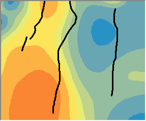
The Kernel Interpolation With Barriers predictions with absolute barriers, left, and without, right, are compared below. Notice how the contours change abruptly at the barriers in the graphic on the left, but the contours flow smoothly over the barriers in the graphic on the right.

Kernel Interpolation predictions with absolute barriers.

Kernel Interpolation predictions without absolute barriers.

Models based on the shortest distance between points may be preferable in hydrological and meteorological applications.

Kernel Functions

Kernel functions: for all formulas below, r is a radius centered at point s and h is the bandwidth.

• Exponential:

  

• Gaussian:

  

• Quartic:

  

• Epanechnikov:

  

• PolynomialOrder5:

  

• Constant:

  

  where I(expression) is an indicator function that takes a value of 1 if expression is true and a value of 0 if expression is false.

The bandwidth parameter applies to all kernel functions except Constant. Exponential, Gaussian, and Constant kernel functions additionally support a smooth searching neighborhood in order to limit the range of the kernel.

References and further reading

Fan, J. and Gijbels, I. (1996). Local Polynomial Modelling and Its Applications, Chapman & Hall. London.

Hoerl, A.E. and Kennard, R.W. (1970), Ridge regression: biased estimation for nonorthogonal problems, Technometrics, 12, 55-67.

Yan, Xin. (2009) Linear regression analysis : theory and computing. Published by World Scientific Publishing Co. Pte. Ltd. 5 Toh Tuck Link, Singapore 596224.