Components of geostatistical models

Disponible avec une licence Geostatistical Analyst.

Geostatistical (kriging) models comprise several components: examining the data, calculating the empirical semivariogram or covariance values, fitting a model to the empirical values, generating the matrices of kriging equations, and solving them to obtain a predicted value and the error (uncertainty) associated with it for each location in the output surface.

Calculate the empirical semivariogram

Kriging, like most interpolation techniques, is built on the basic principle that things that are close to one another are more alike than those farther away from each other (quantified here as spatial autocorrelation). The empirical semivariogram is a means to explore this relationship. Pairs that are close in distance should have a smaller difference than those farther away from one another. The extent to which this assumption is true can be examined in the empirical semivariogram.

Fit a model

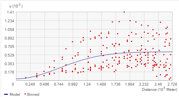
Fitting is done by defining a model that provides the best fit through the points. That is, you need to find a line such that the weighted squared difference between each point and the line is as small as possible. This is referred to as the weighted least-squares fit. This model quantifies the spatial autocorrelation in your data. The image below shows the empirical semivariances (red dots) and the model that best represents the points (blue line):

Create the matrices

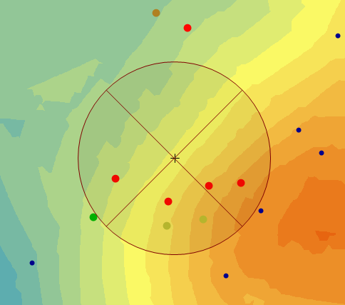
The equations for kriging are contained in matrices and vectors that depend on the spatial autocorrelation among the measured sample locations and prediction location. The autocorrelation values come from the semivariogram model. The matrices and vectors determine the kriging weights that are assigned to each measured value in the searching neighborhood.

Make a prediction

From the kriging weights for the measured values, the software calculates a prediction for the location with the unknown value.