Geostatistical Analyst のライセンスで利用可能。
Indicator kriging assumes the model
I(s) = µ + ε(s),where µ is an unknown constant and I(s) is a binary variable. The creation of binary data may be through the use of a threshold for continuous data, or it may be that the observed data is 0 or 1. For example, you might have a sample that consists of information on whether or not a point is forest or nonforest habitat, where the binary variable indicates class membership. Using binary variables, indicator kriging proceeds the same as ordinary kriging.
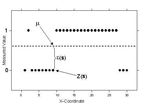
In the following figure, the data has been converted to binary values using the threshold shown in Understanding thresholds.

The observed binary data is given by the open squares. The unknown mean for all indicator variables is shown by the dashed line, and it is µ. This can be compared to ordinary kriging. As with ordinary kriging, you assume that ε(s) is autocorrelated. Notice that because the indicator variables are 0 or 1, the interpolations will be between 0 and 1, and predictions from indicator kriging can be interpreted as probabilities of the variable being 1 or being in the class that is indicated by 1. If a threshold was used to create the indicator variable, the resulting interpolation map would show the probabilities of exceeding (or being below) the threshold.
It is possible to create several indicator variables for the same dataset by choosing multiple thresholds. In this case, one threshold creates the primary indicator variable, and the other indicator variables are used as secondary variables in cokriging.
Indicator kriging can use either semivariograms or covariances, which are the mathematical forms you use to express autocorrelation.