Geostatistical Analyst のライセンスで利用可能。
Ordinary kriging assumes the model
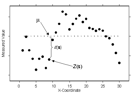
Z(s) = µ + ε(s),where µ is an unknown constant. One of the main issues concerning ordinary kriging is whether the assumption of a constant mean is reasonable. Sometimes there are good scientific reasons to reject this assumption. However, as a simple prediction method, it has remarkable flexibility. The following figure is an example in one spatial dimension:

It looks like the data is elevation values collected from a line transect through a valley and over a mountain. It also looks like the data is more variable on the left and becomes smoother on the right. In fact, this data was simulated from the ordinary kriging model with a constant mean µ. The true but unknown mean is given by the dashed line. Thus, ordinary kriging can be used for data that seems to have a trend. There is no way to decide, based on the data alone, whether the observed pattern is the result of autocorrelation—among the errors ε(s) with µ constant—or trend, with µ(s) changing with s.
Ordinary kriging can use either semivariograms or covariances (which are the mathematical forms you use to express autocorrelation), use transformations and remove trends, and allow for measurement error.