Available with Geostatistical Analyst license.
Introduction
Empirical Bayesian kriging (EBK) is a geostatistical interpolation method that automates the most difficult aspects of building a valid kriging model. Other kriging methods in Geostatistical Analyst require you to manually adjust parameters to receive accurate results, but EBK automatically calculates these parameters through a process of subsetting and simulations.
Empirical Bayesian kriging also differs from other kriging methods by accounting for the error introduced by estimating the underlying semivariogram. Other kriging methods calculate the semivariogram from known data locations and use this single semivariogram to make predictions at unknown locations; this process implicitly assumes that the estimated semivariogram is the true semivariogram for the interpolation region. By not taking the uncertainty of semivariogram estimation into account, other kriging methods underestimate the standard errors of prediction.
Empirical Bayesian kriging is offered in the Geostatistical Wizard and as a geoprocessing tool.
Advantages and disadvantages
Empirical Bayesian kriging has a number of advantages and disadvantages compared to other interpolation methods.
Advantages
- Requires minimal interactive modeling.
- Standard errors of prediction are more accurate than other kriging methods.
- Allows accurate predictions of moderately nonstationary data.
- More accurate than other kriging methods for small datasets.
Disadvantages
- Processing time rapidly increases as the number of input points, the subset size, or the overlap factor increase. Applying a transformation will also increase processing time, particularly if K-Bessel or K-Bessel Detrended is chosen for the semivariogram model type. These parameters are described in subsequent sections of this topic.
- Processing is slower than other kriging methods, especially when outputting to raster.
- Cokriging and anisotropic corrections are unavailable.
- The Log Empirical transformation is particularly sensitive to outliers. If you use this transformation with data that contains outliers, you may receive predictions that are orders of magnitude larger or smaller than the values of your input points. This parameter is described in the Transformations section below.
Semivariogram estimation
Unlike other kriging methods (which use weighted least squares), the semivariogram parameters in EBK are estimated using restricted maximum likelihood (REML). Due to the computational limitations of REML for large datasets, the input data is first divided into overlapping subsets of a specified size (defaulted to 100 points per subset). In each subset, semivariograms are estimated in the following way:
- A semivariogram is estimated from the data in the subset.
- Using this semivariogram as a model, new data is unconditionally simulated at each of the input locations in the subset.
- A new semivariogram is estimated from the simulated data.
- Steps 2 and 3 are repeated a specified number of times. In each repetition, the semivariogram estimated in step 1 is used to simulate a new set of data at the input locations, and the simulated data is used to estimate a new semivariogram.
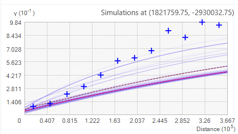
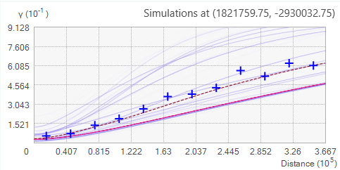
This process creates a large number of semivariograms for each subset, and when they are plotted together, the result is an empirical distribution of semivariograms that are shaded by density (the darker the blue color, the more semivariograms pass through that region). The empirical semivariances are represented by blue crosses. In addition, the median of the distribution is colored with a solid red line, and the 25th and 75th percentiles are colored with red dashed lines, as shown below.
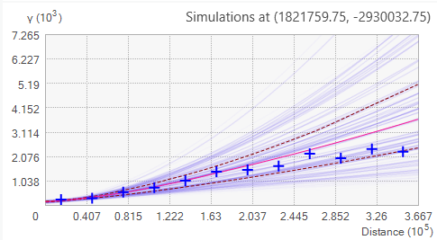
The number of simulated semivariograms per subset is defaulted to 100, and each of these semivariograms is an estimate of the true semivariogram for the subset.
For each prediction location, the prediction is calculated using a new empirical semivariogram distribution that is generated by merging the individual semivariograms from the semivariogram distributions in the point's neighborhood. For example, if a prediction location has neighbors in three subsets (as specified by the searching neighborhood), the prediction will be calculated using the simulated semivariograms from each of the three subsets. The semivariograms from each subset are weighted by the number of neighbors they contribute to the prediction. This allows subsets contributing more neighbors to have more influence on the predicted value.
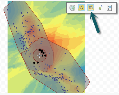
When empirical Bayesian kriging is performed in the Geostatistical Wizard, you are able to see the subsets that were used to calculate the predicted value. In the image below, the prediction location is the center of the crosshairs on the preview surface. The small circle around the crosshairs is the search neighborhood, and the two large, overlapping polygons show the points contained in the two subsets that were used to calculate the prediction. In this example, points in the middle of the map are contained in both subsets. You can turn these polygon visualizations on and off with the button indicated by the arrow:
Kriging model
Empirical Bayesian kriging differs from other kriging methods in Geostatistical Analyst by using an intrinsic random function as the kriging model.
Other kriging models assume that the process follows an overall mean (or specified trend) with individual variations around this mean. Large deviations are pulled back toward the mean, so values never deviate too far. However, EBK does not assume a tendency toward an overall mean, so large deviations are just as likely to get larger as they are to get smaller. Hence, intrinsic random functions inherently correct for trends in the data.
Semivariogram model
For a given distance h, empirical Bayesian kriging supports the following semivariograms:
- Power
- γ(h)= Nugget + b|h|α
- Linear
- γ(h)= Nugget + b|h|
- Thin Plate Spline
- γ(h)= Nugget + b|h2|*ln(|h|)
The Nugget and b (slope) must be positive, and α (power) must be between 0.25 and 1.75. Under these restrictions, the parameters are estimated using REML. These semivariogram models do not have a range or sill parameter because the functions have no upper bound.
In EBK, it's possible to analyze the empirical distribution of the parameter estimates because many semivariograms are estimated at each location. Clicking the Nugget, Slope, or Power tab displays the distributions of the associated parameters. The following graphic shows the distributions of the semivariogram parameters for the simulated semivariograms shown in the previous graphic:
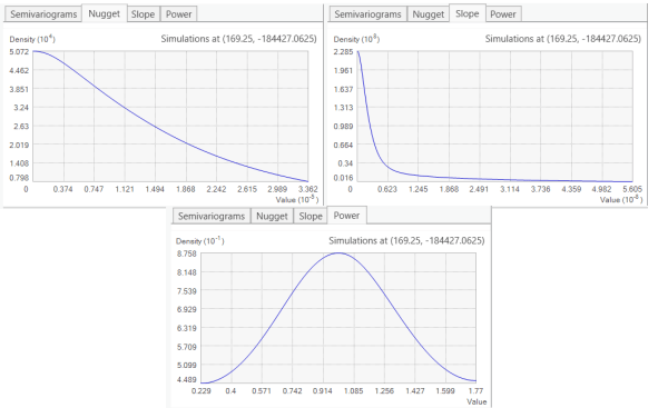
By clicking a different location on the preview surface, the semivariogram distribution and the distributions of the semivariogram parameters are displayed for the new location. If the distributions do not significantly change across the data domain, this suggests that the data is globally stationary. The distributions should change smoothly across the data domain; however, if you see large changes in the distributions over small distances, increasing the value for Overlap Factor can smooth the transitions of the distributions.
Note:
As described in the Transformations section below, applying a transformation changes the kriging model from an intrinsic random function to a simple kriging model, and several additional semivariogram models become available.
Transformations
Empirical Bayesian kriging offers the multiplicative skewing normal score transformation with the choice of two base distributions: Empirical and Log Empirical. The Log Empirical transformation requires all data values to be positive, and it will guarantee that all predictions will be positive. This is appropriate for data such as rainfall that cannot be negative.
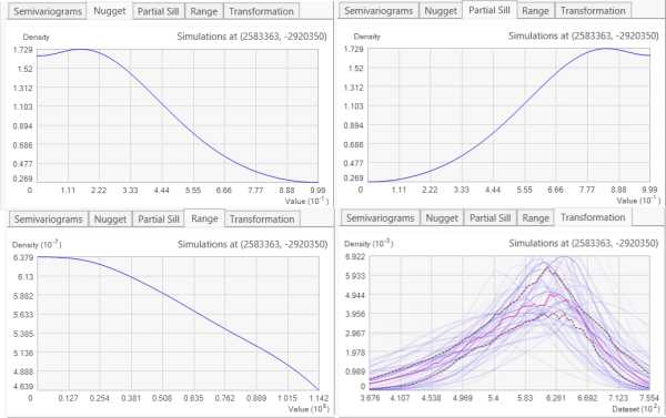
If a transformation is applied, a simple kriging model is used instead of an intrinsic random function. Because of these changes, the parameter distributions change to Nugget, Partial Sill, and Range.
If K-Bessel or K-Bessel Detrended is chosen for the Semivariogram Type, an additional graph for the Shape parameter in K-Bessel will be displayed. An additional Transformation tab also appears that displays the distribution of the fitted transformations (one for each simulation). As with the Semivariograms tab, the transformation distribution is colored by density, and quantile lines are provided.
Semivariograms
All geostatistical methods assume spatial autocorrelation, that closer things are more similar than things that are farther away, and the semivariogram defines how this similarity diminishes over distance. Some semivariograms (Exponential, for example) assume that the similarity diminishes quickly. The Whittle semivariogram model, on the other hand, assumes the similarity diminishes slowly. Even with the same nugget, range, and sill, these two semivariograms will define diminishing similarity in starkly different ways. The key to getting reliable results is to choose the semivariogram that most closely matches how your phenomenon behaves. The semivariogram models available for you depend on your choice of transformation.
If the Transformation is set to None, the following semivariogram models are available:
- Power (default)
- Linear
- Thin Plate Spline
If the Transformation is set to Empirical or Log Empirical, the following semivariogram models are available:
- Exponential (default)
- Exponential Detrended
- Whittle
- Whittle Detrended
- K-Bessel
- K-Bessel Detrended
The three detrended semivariogram models are the same as their nondetrended counterparts, except that a first-order trend removal will be applied. Removing trend has a negligible effect on calculation speed.
Advantages and disadvantages of each model
Each semivariogram has advantages and disadvantages. When choosing a semivariogram, the calculation time and the flexibility of the model (the ability to accurately accommodate a broad range of datasets) should be taken into account:
- Power
- Advantages: Relatively fast and flexible. Generally a safe choice that balances performance and accuracy.
- Disadvantages: Less flexible and slower than other choices.
- Linear
- Advantages: Very fast.
- Disadvantages: Least flexible model.
- Thin Plate Spline
- Advantages: Very fast. Works best when strong trends are present.
- Disadvantages: Less flexible, particularly when no trend is present.
- Exponential
- Advantages: Offers a flexible transformation. Faster than K-Bessel and K-Bessel Detrended.
- Disadvantages: Shape of the semivariogram is not flexible. Slow compared to Power, Linear, and Thin Plate Spline.
- Exponential Detrended
- Advantages: Offers a flexible transformation. Faster than K-Bessel and K-Bessel Detrended. Removes first order trend.
- Disadvantages: Shape of the semivariogram is not flexible. Slow compared to Power, Linear, and Thin Plate Spline.
- Whittle
- Advantages: Offers a flexible transformation. Faster than K-Bessel and K-Bessel Detrended.
- Disadvantages: Shape of the semivariogram is not flexible. Slow compared to Power, Linear, and Thin Plate Spline.
- Whittle Detrended
- Advantages: Offers a flexible transformation. Faster than K-Bessel and K-Bessel Detrended. Removes first order trend.
- Disadvantages: Shape of the semivariogram is not flexible. Slow compared to Power, Linear, and Thin Plate Spline.
- K-Bessel
- Advantages: Most flexible and accurate.
- Disadvantages: Takes the longest to calculate.
- K-Bessel Detrended
- Advantages: Most flexible and accurate. Removes first order trend.
- Disadvantages: Takes the longest to calculate.
Choosing a semivariogram
The choice of the semivariogram should be clear most of the time, based on the following criteria:
- If you are willing to wait to get the most accurate results, K-Bessel or K-Bessel Detrended should be chosen. The presence or absence of trend should determine which one.
- If you need results quickly and are willing to sacrifice some accuracy, Linear or Thin Plate Spline should be chosen. If there is no trend or the trend is weak, Linear is a better choice.
- If you need a balance of accuracy and speed, Power is a good choice.
- If a transformation is required, but you cannot afford to wait a long time for output, Exponential or Whittle (or their detrended counterparts) should be chosen. You should choose the one that best matches the empirical semivariances in the Geostatistical Wizard (described below). Crossvalidation should also be taken into account.
If you are trying to choose between Exponential, Whittle, and their detrended counterparts, you should choose the semivariogram that provides the best visual fit to the empirical semivariances (the blue crosses in the graphics below). Ideally, the empirical semivariances should fall in the middle of the semivariogram spectrum. For example, in the following graphic, the blue crosses do not fall in the middle of the semivariogram spectrum (most fall toward the top of the spectrum):
Instead, the following semivariogram should be preferred because the blue crosses fall in the middle of the semivariogram spectrum:
Distance calculations for data in geographic coordinates
If your input data is in a geographic coordinate system, distances will be calculated using chordal distance. The chordal distance between any two points is the straight-line distance that connects the two points. This line will go through the earth rather than along its surface. To visualize this, imagine shining a flashlight through a transparent sphere. The length of the beam of light between the point where the light enters and exits the sphere is the chordal distance between these two points. The primary benefit of using chordal distance over geodesic distance is that it is less computationally intensive. Additionally, there is only limited theory about performing kriging on spheroids.
Note:
Because chordal distances are not good approximations of geodesic distances for distances over 30 decimal degrees, the search radius cannot exceed 15 decimal degrees (thus, the diameter cannot exceed 30 degrees), and any location that does not have any neighbors within 15 decimal degrees will be calculated as NoData. Additionally, some semivariogram models require fitting a flat plane to each subset to perform trend removal. This plane cannot be accurately created for subsets whose extent exceeds 30 decimal degrees, so the extent of individual subsets is restricted to 30 degrees for the following semivariogram models:
- Thin Plate Spline
- Exponential Detrended
- Whittle Detrended
- K-Bessel Detrended
Previous versions of ArcGIS treated geographic coordinates as square coordinates and calculated the Euclidean distance between the points. However, a 1 degree by 1 degree cell is not actually a square, so this distance will be distorted. This distortion gets worse as you move farther north or south from the equator.
Additional parameters for empirical Bayesian kriging
Empirical Bayesian kriging employs three parameters that do not appear in other kriging methods:
- Maximum number of points in each local model—Specifies the number of points in each subset. The larger the subset size, the longer EBK will take to calculate.
- Local model area overlap factor—Specifies the degree of overlap between subsets. Each input point can fall into several subsets, and the overlap factor specifies the average number of subsets that each point will fall into. For example, an overlap factor of 1.5 means that about half the points will be used in one subset and half will be used in two subsets. A higher value for the overlap factor makes the output surface smoother, but it also increases processing time.
- Number of simulated semivariograms—Specifies the number of semivariograms that will be simulated for each subset. More simulations will cause the predictions to be more precise, but processing time will also increase.
References
- Chilès, J-P., and P. Delfiner (1999). Chapter 4 of Geostatistics: Modeling Spatial Uncertainty. New York: John Wiley & Sons, Inc.
- Krivoruchko K. (2012). "Empirical Bayesian Kriging," ArcUser Fall 2012.
- Krivoruchko K. (2012). "Modeling Contamination Using Empirical Bayesian Kriging," ArcUser Fall 2012.
- Krivoruchko K. and Gribov A. (2014). "Pragmatic Bayesian kriging for non-stationary and moderately non-Gaussian data," Mathematics of Planet Earth. Proceedings of the 15th Annual Conference of the International Association for Mathematical Geosciences, Springer 2014, pp. 61-64.
- Krivoruchko K. and Gribov A. (2019). "Evaluation of empirical Bayesian kriging," Spatial Statistics Volume 32. https://doi.org/10.1016/j.spasta.2019.100368.
- Pilz, J., and G. Spöck (2007). "Why Do We Need and How Should We Implement Bayesian Kriging Methods," Stochastic Environmental Research and Risk Assessment 22 (5):621–632.