The Forest-based and Boosted Classification and Regression tool trains a model based on known values provided as part of a training dataset. The model can then be used to predict unknown values in a dataset that has the same explanatory variables. The tool creates models and generates predictions using one of two supervised machine learning methods: an adaptation of the random forest algorithm, developed by Leo Breiman and Adele Cutler, and XGBoost, a popular boosting method developed by Tianqi Chen and Carlos Guestrin.
The forest-based model creates many independent decision trees, collectively called an ensemble or a forest. Each decision tree is created from a random subset of the training data and explanatory variables. Each tree generates its own prediction and is used as part of an aggregation scheme to make the final predictions. The final predictions are not based on any single tree but rather on the entire forest. This helps avoid overfitting the model to the training dataset.
The gradient boosted model creates a series of sequential decision trees. Each subsequent decision tree is built to minimize the error (bias) of the previous decision tree, so the gradient boosted model combines several weak learners to become a strong prediction model. The gradient boosted model incorporates regularization and early stopping, which can prevent overfitting the model to the training dataset.
Both model types can be constructed to predict either a categorical variable (binary classification and multiclass classification) or a continuous variable (regression). When the variable to predict is categorical, the model that is constructed is based on classification trees; when it is continuous, the model that is constructed is based on regression trees.
Potential applications
The following are potential applications for this tool:
- Given data on occurrence of seagrass, several environmental explanatory variables represented as both attributes and rasters, and the distances to factories upstream and major ports, future seagrass occurrence can be predicted based on future projections for those same environmental explanatory variables.
- Suppose you have data on the crop yield at hundreds of farms across the country, data on the characteristics of each farm such as the number of employees and acreage, and several rasters that represent the slope, elevation, rainfall, and temperature at each farm. Using these pieces of data, you can create a model that will predict crop yield. If you then provide the model with a set of features that represent farms with all the same explanatory variables, you can make a prediction about crop yield at each farm.
- Housing values can be predicted based on the prices of houses that have been sold in the current year. The sale price of homes sold along with information about the number of bedrooms, distance to schools, proximity to major highways, average income, and crime counts can be used to predict sale prices of similar homes.
- Land-use types can be classified using training data, a combination of raster layers, including multiple individual bands, and products such as NDVI.
- Given information on the blood lead levels of children and the tax parcel ID of their homes, parcel-level attributes such as age of home, census-level data such as income and education levels, and national datasets reflecting toxic release of lead and lead compounds, the risk of lead exposure for parcels without blood lead level data can be predicted. These risk predictions could drive policies and education programs in the area.
Train a model
The first step in using the Forest-based and Boosted Classification and Regression tool is training a model for prediction. Training builds a forest or sequence of trees that establishes a relationship between the explanatory variables and the Variable to Predict parameter. Whether you choose the Train only, Predict to features, or Predict to raster option, the tool begins by constructing a model based on the Variable to Predict parameter and any combination of the Explanatory Training Variables, Explanatory Training Distance Features, and Explanatory Training Rasters (available with a Spatial Analyst extension license) parameters.
Explanatory Training Variables
A common source of explanatory variables to train the model with is the other fields in the training dataset that contains the Variable to Predict parameter. Regardless of whether you choose to predict a continuous variable or a categorical variable, each field in the Explanatory Training Variables values can be either continuous or categorical. If the trained model is also being used to make predictions, each of the provided Explanatory Training Variables values must be available for both the training dataset and the prediction dataset.
Explanatory Training Distance Features
Although Forest-based and Boosted Classification and Regression is not a spatial machine learning tool, one way to leverage the power of space in your analysis is to use distance features. For example, if you are modeling the performance of a series of retail stores, a variable representing the distance to highway on-ramps or the distance to the closest competitor could be critical to producing accurate predictions. Similarly, if modeling air quality, an explanatory variable representing distance to major sources of pollution or distance to major roadways would be critical. Distance features are used to automatically create explanatory variables by calculating a distance from the provided features to the Input Training Features value. Distances will be calculated from each feature of the Input Training Features value to the nearest feature of the input Explanatory Training Distance Features value. If the input Explanatory Training Distance Features value contains polygons or lines, the distance attributes are calculated as the distance between the closest segments of the pair of features. However, distances are calculated differently for polygons and lines. See How proximity tools calculate distance for details.
Explanatory Training Rasters
The Explanatory Training Rasters values can also be used to train the model. This allows you to use imagery, DEMs, population density models, environmental measurements, and many other data sources in the model. Regardless of whether you choose to predict a continuous variable or a categorical variable, each of the Explanatory Training Rasters values can be either continuous or categorical. The Explanatory Training Rasters parameter is only available if you have a Spatial Analyst license.
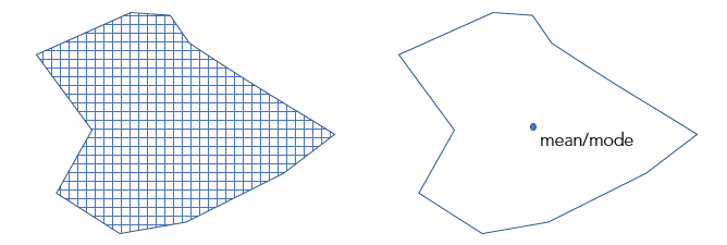
If the features in the Input Training Features value are points and you have specified a Explanatory Training Rasters value, the tool drills down to extract explanatory variables at each point location. For multiband rasters, only the first band is used. For mosaic datasets, use the Make Mosaic Layer tool first. If your Input Training Features value contains polygons, the Variable to Predict value is categorical, and you've specified a Explanatory Training Rasters value, the Convert Polygons to Raster Resolution for Training parameter is enabled and active. If this option is checked, each polygon is divided into points at the centroid of each raster cell whose centroid falls within the polygon and the polygons are treated as a point dataset. The raster values at each point location are then extracted and used to train the model. The model is no longer trained on the polygon; rather, the model is trained on the raster values extracted for each cell centroid. A bilinear sampling method is used for numeric variables and the nearest method is used for categorical variables. The default cell size of the converted polygons will be the maximum cell size of input rasters. You can change this size using the Cell Size environment setting. If Convert Polygons to Raster Resolution for Training parameter is not checked, one raster value for each polygon will be used in the model. Each polygon is assigned the average value for continuous rasters and the majority for categorical rasters.
Predict using a model
It is recommended that you start with the Train only option; evaluate the results of the analysis; adjust the variables included and the advanced parameters as necessary; and once a good model is found, rerun the tool to predict to either features or a raster. You can use the tool to help you find the best model. Check the Optimize parameter check box and select an Optimization Model parameter option.
Learn more about parameter optimization
When moving on to prediction, it is recommended that you change the Training Data Excluded for Validation (%) parameter to 0 percent so that you can include all the available training data in the final model used to make predictions. You can make predictions in the following ways:
Predict in the same study area
When predicting to features in the same study area, each prediction feature must include all the associated explanatory variables (fields). The extent of the features must overlap with the extent of the Explanatory Training Distance Features and Explanatory Training Rasters values.
When predicting to a raster in the same study area using the provided Explanatory Training Rasters value, the extent of the prediction raster will be the overlapping extent of all explanatory rasters.
Predict to a different study area
When predicting to features in a different study area, each prediction feature must include all of the associated explanatory variables (fields), explanatory distance features, and explanatory rasters. These new distance features and rasters must be available for the new study area and correspond to the Explanatory Training Distance Features and Explanatory Training Rasters values.
When predicting to a raster in a different study area, new explanatory prediction rasters must be provided and matched to their corresponding Explanatory Training Rasters value. The extent of the resulting Output Prediction Raster value will be the overlapping extent of all the provided explanatory prediction rasters.
Predict to a different time period by matching the explanatory variables used for training to variables with projections in the future
When predicting to a future time period, whether predicting to features or a raster, each projected explanatory prediction variable (fields, distance features, and rasters) must be matched to the corresponding explanatory training variables.
The Forest-based and Boosted Classification and Regression tool does not extrapolate, so the corresponding explanatory variable fields, distance features, and explanatory rasters in the Input Prediction Features value cannot have a dramatically different range of values or categories than those used to train the model.
Predict to features
A model that has been trained using any combination of the Explanatory Training Variables, Explanatory Training Distance Features, and Explanatory Training Rasters parameter values can be used to predict to either points or polygons in either the same or a different study area. Predicting to features requires that every feature receiving a prediction have a value for each field, distance feature, and raster used to train the model.
If the field names in the Input Training Features and Input Prediction Features values do not match, a Match Explanatory Variables parameter is enabled and active. When matching explanatory variables, the field specified by the Prediction and Training parameter values must be of the same type. For example, a double field in the Input Training Features value must be matched to a double field in the Input Prediction Features value. If you predict to a different study area or a different time period, you can use distance features or rasters that were not used for training the model. A Match Distance Features and Match Explanatory Rasters parameter will be enabled and active.
Predicting to rasters
Using a model that has been trained using only Explanatory Training Rasters, you can predict to a raster in either the same or a different study area. If you predict to either a different study area or time period, you can use prediction rasters that were not used for training the model. A Match Explanatory Rasters parameter will be enabled and active. An Output Prediction Raster can be created with a Spatial Analyst license by choosing the Predict to raster option as the Prediction Type parameter value.
Evaluate a model
Once this tool creates a model, you can evaluate that model. This tool creates messages and charts to help you understand the characteristics of the model and to evaluate its performance.
Geoprocessing messages
You can access the messages by hovering over the progress bar, clicking the pop-out button, or expanding the messages section in the Geoprocessing pane. You can also access the messages for a previous run of this tool in the geoprocessing history. The messages include information about the characteristics of your model, Out of Bag (OOB) errors, variable importance, training and validation diagnostics, and diagnostics on the explanatory variable range.
Model Characteristics table
The Model Characteristics table contains information on several important aspects of your forest or boosted model, some of which are selected using the parameters in the Advanced Model Options drop-down menu and some of which are data driven. Data-driven model characteristics are important to understand when optimizing the performance of the model. The Tree Depth Range reports the minimum and maximum tree depth found in the forest or sequence of trees. The maximum depth is set by the Maximum Tree Depth parameter; however, any depth less than the maximum is possible. The Mean Tree Depth value reports the average depth of trees in the forest or sequence of trees. If the Maximum Tree Depth parameter was set to 100, but the Tree Depth Range and Mean Tree Depth values report smaller numbers, setting a smaller maximum tree depth may improve the performance of the model, because it decreases the chances of overfitting the model to the training data. The Number of Randomly Sampled Variables value reports the number of randomly selected variables that are used for any given tree in the model. Each tree will have a different combination of variables, but the same number of variables. By default, the number is based on a combination of the number of features and the number of variables available. For regression, it is one-third of the total number of explanatory variables (including features, rasters, and distance features). For classification, it is the square root of the total number of variables. If the Model Type parameter is specified as Forest-based, the Model Characteristics table will include Number of Trees, Leaf Size, Tree Depth Range, Mean Tree Depth, % of Training Available per Tree, Number of Randomly Sampled Variables, and % of Training Data Excluded for Validation values. If the Model Type parameter is specified as Gradient Boosted, four additional values are listed in the table: L2 Regularization (Lambda), Minimum Loss Reduction for Splits (Gamma), Learning Rate (Eta), and Maximum Number of Bins for Searching Splits.

Model Out of Bag Errors table
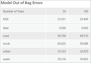
If the Model Type parameter is specified as Forest-based, the geoprocessing messages will include a Model Out of Bag Errors table. OOB errors help you evaluate the accuracy of the model. Both MSE (mean squared error) and % of variation explained are based on the ability of the model to accurately predict the Variable to Predict value based on the observed values in the training dataset. OOB is a prediction error calculated using the data that is a part of the training dataset that is not seen by a subset of the trees in the forest. If you want to train a model on 100 percent of your data, you will rely on OOB to assess the accuracy of your model. These errors are reported for half the number of trees used and the total number of trees used to help evaluate whether increasing the number of trees is improving the performance of the model. If the errors and percentage of variation explained are similar for both numbers of trees, it is an indicator that a smaller number of trees can be used with minimal impact on model performance. However, it is best practice to use as many trees as your machine allows. A higher number of trees in the forest will result in more stable results and a model that is less prone to noise in the data and sampling scheme.

If the variable to predict is categorical (indicated by the Treat Variable as Categorical parameter value), OOB errors are calculated based on the percent of incorrect classifications for each category among trees that did not see a subset of the trees in the forest. The percentage of incorrect OOB classifications for each category is printed in the geoprocessing messages. The MSE of the classifications is also printed and can be interpreted as the overall proportion of incorrect OOB classifications among all categories. If the Number of Trees value is small, it is possible that one or more categories will never be used to train the data. In this case, the OOB error will be 100 percent.
Top Variable Importance table
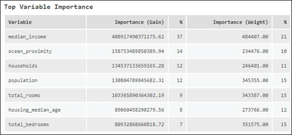
Another factor that impacts the performance of the model is the explanatory variables used. The Top Variable Importance table lists the explanatory variables with the top 20 importance scores. Variable importance is a diagnostic that helps you understand which variables are driving the results of the model. A best practice is to first use all the data for training and explore the importance of each explanatory variable. Then you can use variable importance to create a simpler (parsimonious) model that only includes the explanatory variables that are detected to be meaningful.

When the Model Type parameter value is Forest-based, importance is calculated using Gini coefficients, which can be thought of as the number of times a variable is responsible for a split and the impact of that split divided by the number of trees. Each split is an individual decision in a decision tree.
When the Model Type parameter value is Gradient Boosted, variable importance is calculated in three different ways: Importance (Gain), Importance (Weight), and Importance (Cover). Importance (Gain) represents the relative contribution of an explanatory variable to the model. The Importance (Gain) is calculated by summing the gain of all the splits where an explanatory variable is used. Importance (Weight) represents the number of times an explanatory variable is used across all splits. Importance (Cover) represents the number of observations across all the trees that are defined by an explanatory variable. Importance (Cover) is not listed in the geoprocessing messages; however, if the Output Variable Importance Table parameter is specified, Importance (Cover) will be a field in the table and can be displayed in the Summary of Variable Importance chart. These two outputs can be accessed from the Contents pane. If the Number of Runs for Validation value is greater than 1, the tool will calculate the set of variable importance for each iteration. The geoprocessing messages will list the set of variable importance of the iteration with an R-Squared or accuracy that is closest to the median R-Squared or accuracy. To review all sets of variable importance, specify an Output Variable Importance Table parameter value.
Validation and training data diagnostics
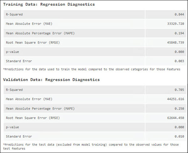
Another important way to evaluate the performance of the model is to use the model to predict the value of features then to compare those predicted values to the observed values and calculate diagnostics. This is performed on the training data and the testing (validation) data. By default, this tool will exclude 10 percent of the features in the Input Training Features value for testing. However, this can be controlled using the Training Data Excluded for Validation (%) parameter. One disadvantage of OOB is that it uses a subset of the forest (trees that have not used a specific feature from the training dataset) as opposed to using the entire forest. By excluding some data for validation, error metrics can be assessed for the entire model. The geoprocessing messages report the diagnostics in the validation data diagnostics table and the training data diagnostics table. These diagnostics can help you understand how well the model fits the data.
When predicting a continuous variable, the observed value for each of the train features and test features is compared to the predictions for those features based on the trained model and an associated R-Squared, Mean Absolute Error (MAE), Mean Absolute Percentage Error (MAPE), Symmetric Mean Absolute Percentage Error (SMAPE), Root Mean Square Error (RMSE), p-value, and Standard Error values are reported in the geoprocessing messages. These diagnostics will change each time you run through the training process because the selection of the train and test dataset is random. To create a model that does not change with every run, you can set a seed in the Random Number Generator environment setting.
When predicting a categorical variable, Sensitivity, Accuracy, F1-Score, and MCC are reported in the geoprocessing messages. These diagnostics are calculated using the table specified by the Output Classification Performance Table (Confusion Matrix) parameter, which tracks the number of times a category of interest is correctly and incorrectly classified and the number of times other categories are misclassified as the category of interest. Sensitivity for each category is reported as the percentage of times features with an observed category were correctly predicted for that category. For instance, if you are predicting Land and Water, and Land has a sensitivity of 1.00, every feature that should have been marked Land was correctly predicted. If, however, a Water feature was incorrectly marked Land, it would not be reflected in the sensitivity number for Land. This would be reflected in Water's sensitivity number because one of the water features was not correctly classified.
The accuracy diagnostic takes into account both how well features with a particular category are predicted and how often other categories are misclassified as the category of interest. It gives an estimate of how frequently a category is identified correctly among the total number of observations for that category. When classifying a variable with only two classes, the accuracy measure will be the same for each class, but the sensitivity can differ. When classifying a variable with more than two classes, both sensitivity and accuracy can differ between classes. 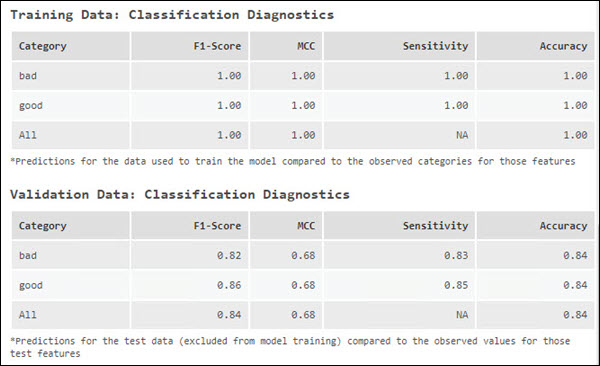
| Diagnostic | Description | |||||||||||||||||||||||||
|---|---|---|---|---|---|---|---|---|---|---|---|---|---|---|---|---|---|---|---|---|---|---|---|---|---|---|
R-Squared | R-Squared is a measure of goodness of fit. It is the proportion of dependent variable variance accounted for by the regression model. The value varies from 0.0 to 1.0 and a higher value denotes a better model. Increasing the number of explanatory variables will always increase R2. The increase may not reflect an improvement in the model fit but rather how R2 is calculated. | |||||||||||||||||||||||||
Mean Absolute Error (MAE) | MAE is the average of the absolute difference between the actual values and predicted values of the Variable of Interest parameter. A value of 0 means the model correctly predicted every observed value. MAE is in the units of the variable of interest, so it cannot be compared across different models. | |||||||||||||||||||||||||
Mean Absolute Percentage Error (MAPE) | MAPE is similar to MAE in that it represents the difference between the actual values and predicted values. However, while MAE represents the difference in the original units, MAPE represents the difference as a percentage. MAPE is a relative error, so it is a better diagnostic when comparing different models. Due to how MAPE is calculated, it cannot be used if any of the actual values are 0. If the actual values are close to 0, MAPE will go to infinity. Another limitation of MAPE is that it is asymmetrical. For example, if there are two cases where the difference between the actual values and the predicted values are the same, the case where the actual value is smaller will contribute more to MAPE. | |||||||||||||||||||||||||
Symmetric Mean Absolute Percentage Error (SMAPE) | As with MAPE, SMAPE represents the difference between the actual values and the predicted values as a percentage, but SMAPE addresses the asymmetric problem in its calculation. | |||||||||||||||||||||||||
Root Mean Square Error (RMSE) | RMSE is the square root of mean square error (MSE), which is the square root of the averaged squared difference between the actual values and the predicted values. As with MAE, RMSE represents the average model prediction error in the units of the variable of interest; however, RMSE is more sensitive to large errors. To avoid a model that has a large difference between the actual values and the predicted values, you can use RMSE to evaluate the model. | |||||||||||||||||||||||||
p-value | P-value is a statistical measure that is used to validate a hypothesis that the observations are not correlated with the predictions. When the p-value is less that 0.05, the correlation between observations and predictions is significant. | |||||||||||||||||||||||||
Standard Error | This is the standard error of the regression slope. It represents how far the observed values deviate from the predicted values on average. | |||||||||||||||||||||||||
F1-Score | F1-score is a measure of model performance. It is a value between 0 and 1 that is calculated for each class. Higher F1-Scores indicate a better model. The F1-Score of all the classes (macro F1-Score) is the mean of the F1-Score of the individual classes. If the number of features in each class is uneven, F1-Score is a better metric to evaluate the model than accuracy. F1-Score maximizes precision and recall. Precision is calculated by dividing the number of times a category of interest was correctly classified by the total number of times the category of interest was predicted. Recall is calculated by dividing the number of times a category of interest was correctly classified by the number of features with that category. F1-Score is then calculated as follows:
In the following table, class A was correctly classified 25 times and predicted 30 times (25 + 4 + 1), so the precision of class A is 25/30. There are 25 features with class A (25 + 0 + 0) , so the recall of class A is 25/25. The F1-Score of class A is 0.909.
| |||||||||||||||||||||||||
MCC | Similar to F1-Score, MCC summarizes the confusion matrix using a value between -1 and 1. A value of -1 means that the model misclassified every feature, and a value of 1 indicates that the model correctly categorized every feature. MCC is different from F1-Score in that MCC also considers the number of times the category of noninterest was predicted, so MCC will only be high when the model performs well on the category of interest and the category of noninterest. | |||||||||||||||||||||||||
Sensitivity | Sensitivity is the percentage of times features with an observed category were correctly predicted for that category. It is calculated by dividing the number of times a class of interest was correctly classified by the number of features with that class. In the following table, class A was correctly predicted 25 times and there are 25 features (25 + 0 + 0) with class A, so the sensitivity of class A is 25/25.
| |||||||||||||||||||||||||
Accuracy | Accuracy is the number of times a category is identified correctly among the total number of observations for that category. Accuracy takes into account how well features with a particular category are predicted and how often other categories are correctly identified as not the category of interest. Accuracy is calculated as follows:
where TP means True Positive, TN means True Negative, FP means False Positive, and FN means False Negative. In the following table, for class A, TP is 25, TN is 45 (19 + 3 + 2 + 21), FP is 5 (4 + 1), and FN is 0 (0 + 0). The accuracy of class A is 70/(25+45+5+0) = 0.93. The accuracy of all the classes is (25 + 19 +21)/75 = 0.866.
|
Explanatory Variable Range Diagnostics table
The explanatory range diagnostics can help you evaluate whether the values used for training, validation, and prediction are sufficient to produce a good model and whether you can trust the other model diagnostics. The data used to train a model has a large impact on the quality of the resulting classification and predictions. Ideally, the training data should be representative of the data you are modeling. By default, 10 percent of the features in the Input Training Features value is randomly excluded for validation. This results in a training dataset and a validation dataset. The Explanatory Variable Range Diagnostics table shows the minimum and maximum values of these datasets and, if predicting to features or rasters, of the data used for prediction.
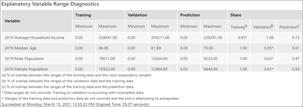
Due to the random nature of how subsets are determined, the values of the variables in the training subset may not be representative of the overall values in the Input Training Features value. For each continuous explanatory variable, the Training column in the Share group indicates the percentage of overlap between the range of values of the training subset and the range of values of all the features in the Input Training Features value. For example, if variable A from Input Training Features had the values 1 through 100 and the training subset had the values 50 through 100, the value for variable A in the Training column in the Share group would be 0.50 or 50 percent. For variable A, 50 percent of the range of values of the Input Training Features is included in the training subset. If the training subset does not cover a wide range of the values found in Input Training Features for each explanatory variable in the model, other model diagnostics may be biased. A similar calculation is performed to produce the Validation column in the Share group of the table. It is important that the range of values used to validate the model covers as much of the range of values used to train the model as possible. For example, if variable B from the training subset had the values 1 through 100 and the validation subset had the values 1 through 10, the Validation column in the Share group for variable B would be 0.10 or 10 percent. This small range of values might be all low values or all high values and would thus bias other diagnostics. If the validation subset held all low values, other model diagnostics such as MSE and percent of variation explained would report how well the model predicts to low values and not to the complete range of values found in the input training features. Additionally, a value greater than 1 indicates that the range of values used for validation is greater than the range of the values in the training subset. Thus, the validation diagnostic will be poor because the random forest and extreme gradient boosted algorithms cannot extrapolate.
The Prediction column in the Share group of the Explanatory Variable Range Diagnostics table is particularly important. Forest-based and gradient boosted models do not extrapolate; they can only classify or predict to a value within the range on which the model was trained. The Prediction column in the Share group is the percentage of overlap between the range of values of the training data and the range of values in the prediction data. A value of 1 indicates that the range of values in the training subset and the range of values being used for prediction are equivalent. A value greater than 1 indicates that the range of the values used for prediction is greater than the range of the values in the training subset. It also indicates that you are attempting to predict to a value on which the model was not trained.
All three share diagnostics are only valid if the ranges of the subsets are coincident. For example, if the validation subset for variable C had the values 1 through 100 and the training subset had the values 90 through 200, they would overlap by 10 percent, but they do not have coincident ranges. In this case, the diagnostic is marked with an asterisk to show noncoincident ranges. Examine the minimum and maximum values to see the extent and direction of nonoverlap. The Prediction column in the Share group is marked with a plus sign (+) if the model is attempting to predict outside the range of the training data.
There are no absolute rules for acceptable values for the Explanatory Variable Range Diagnostics table. The Training and Validation column in the Share group should be as high as possible, given the constraints of your training data. If the Validation column in the Share group is low, consider increasing the value of the Training Data Excluded for Validation (%) parameter. The Prediction column in the Share group should be as close to 1 as possible. If the Prediction column in the Share group is low, consider decreasing the value of the Training Data Excluded for Validation parameter. Also consider running the model multiple times and choose the run that balances the best values of the range diagnostics. The random seed used in each run is reported in the messages.
Additional outputs
The Forest-based and Boosted Classification and Regression tool also produces a variety of tables, charts, and outputs.
Output trained features
The Output Trained Features parameter value will contain the Input Training Features value, including the training dataset and test (validation) dataset, the Explanatory Training Variables parameter value used in the model, predicted values, the probability of the predicted value in classification, and the probability of the other possible values in classification when the Include All Prediction Probabilities parameter is checked. If the variable to predict is continuous, the output will include the Residual and Standardized Residual fields. If the variable to predict is categorical, the output will include the Correctly Classified field. If the model predicts the known category correctly, the feature is labeled Correctly Classified; otherwise, the feature is labeled Misclassified. For regression models, the trained features are symbolized by the standardized residuals of the predictions. For classification, the symbology of the trained features is based on whether the feature is correctly classified.
The fields of the output trained features include the extracted raster values for each Explanatory Training Rasters variable and calculated distance values for each Explanatory Training Distance Features variable. These new fields can be used to rerun the training portion of the analysis without extracting raster values and calculating distance values each time. The Output Trained Features value will also contain predictions for all of the features, including those used for training and those excluded for testing. This can be helpful in assessing the performance of the model. The trained_features field in the Output Trained Features value indicates whether a feature was used for training.
The Output Trained Features value also will include the following charts, if the variable to predict is categorical:
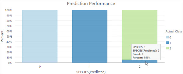
- Prediction Performance—A stacked bar chart. Each bar represents the predicted category, and the color of the subbars reflects the actual category. The size of the subbars reflects the proportion of the features with a given actual class that are within a predicted class. For example, the bar on the right indicates that of the features that are predicted as Species 2, 5.66% had an actual category Species 1.
- Confusion Matrix—A matrix heat chart. The x-axis represents the predicted category of the features in the Input Training Features value and the y-axis represents their actual category. The diagonal cells visualize the number of times the model correctly predicted a category. Higher counts in the diagonal cells indicate that the model performed well. This chart is only produced if the Treat Variable as Categorical parameter is checked.
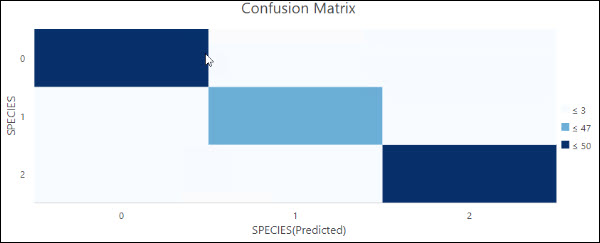
Both charts include the training and testing data. To evaluate how well the model fits the training data, select the features in which the trained_features field is equal to 1, and regenerate this chart. To evaluate how well the model performs on the testing data, select the features in which the trained_features field is equal to 0, and regenerate this chart.
Output Variable Importance Table
The Output Variable Importance Table value contains the explanatory variables used in the model and their importance.
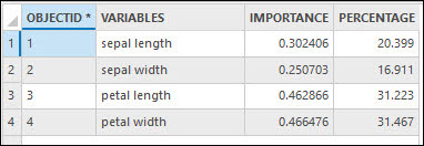

If you specify an Output Variable Importance Table parameter value and the Number of Runs for Validation value is 1, the tool will also output a Summary of Importance Variable chart. If the Model Type parameter value is the Forest-based option, the chart displays the variables used in the model on the y-axis and their importance based on the Gini coefficient on the x-axis . If the Model Type parameter value is the Gradient Boosted option, the importance shown on the x-axis is based on gain values. The explanatory variables are displayed in order of their importance from most (top) to the least (bottom) important.

If you specify an Output Variable Importance Table parameter value and the Number of Runs for Validation value is greater than 1, the Output Variable Importance Table value will include the importance of each explanatory variable for each run and will mark the iteration with the highest accuracy or R2. The set of variable importance printed in the geoprocessing messages is not the set with the best R-Squared or accuracy, but the set with an R2 or accuracy closest to the median R2 or accuracy.

Additionally, if the Number of Runs for Validation value is greater than 1, the tool will output a Distribution of Variable Importance chart. Use this box plot to evaluate the change of variable importance between different runs.
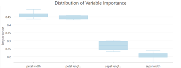
The box plot shows the distribution of variable importance values across all the validation runs. The distribution of variable importance is an indicator of the stability of the trained model. If the importance of a variable is changing broadly across validation runs, this may indicate that the model is unstable. An unstable model can often be improved by increasing the Number of Trees parameter value to capture more complex relationships in the data.
Output Classification Performance Table (Confusion Matrix)
If the variable to predict is categorical, the Output Classification Performance Table (Confusion Matrix) parameter will be available. This table includes all the features in the Input Training Features Excluded for Validation value. Each row represents the actual category and each column represents the predicted category. The table shows the number of true positives (TP), true negatives (TN), false positives (FP), and false negatives (FN) in each category which allows us to calculate several classification diagnostics such as accuracy and sensitivity.
Output predictions
If you use this tool to predict features, the specified Output Predicted Features value will be a feature class with the model's predicted value for each feature. If you predict to a raster, the specified Output Prediction Surface value will be an output raster with the prediction results.
The probabilities of the predicted values are provided when the value to predict is categorical. If the Include All Prediction Probabilities parameter is checked, the probabilities of all other possible values are also included. Probabilities are calculated differently depending on the Model Type parameter value:
- Forest-based—Probabilities are calculated using the percentage of trees voting for each category.
- Gradient-boosted—Probabilities are calculated for each category, individually, by fitting a logistic function, and standardizing probabilities to ensure that they add up to one.
You can use probabilities to measure uncertainty in a prediction. Values closer to 1 are associated with a higher confidence in the prediction. You can also analyze probabilities for a specific class throughout the study area, checking the Include All Prediction Probabilities parameter, and assessing the probability of a particular class across locations of interest.
Advanced Model options
One strength of the forest-based method is in capturing commonalities of weak predictors (or trees). If a relationship is persistently captured by singular trees, it means that there is a strong relationship in the data that can be detected even when the model is not complex. Another strength of both the forest-based and gradient boosted models is that they combine weak predictors (independent trees or a sequence of trees) to create a powerful predictor. Adjusting the model parameters can help create a large number of weak predictors resulting in a powerful model. You can create weak predictors by using less information in each tree. This can be accomplished by using a small subset of the features per tree, a small number of variables per tree, a low tree depth, or any combination of these. The number of trees controls how many of these weak predictors are created and the weaker your predictors (trees), the more trees you need to create a strong model.
The following advanced training and validation options are available in the tool:
- The default Number of Trees parameter value is 100. Increasing the number of trees in the forest or boosted model will generally result in more accurate model predictions, but the model will take longer to calculate. If the Number of Trees parameter value is 0, the model will not be created and the Output Trained Features value will only contain the features from the Input Training Features value and the provided Explanatory Training Variables value.
- Minimum leaf size is the minimum number of observations required to keep a leaf (the terminal node on a tree). The default is 5 for regression and 1 for classification. For very large datasets, increasing the Minimum Leaf Size value will decrease the run time of the tool. If the Minimum Leaf Size value is small (close to the minimum), your model will be prone to noise in your data. For a more stable model, experiment with increasing the Minimum Leaf Size value.
- Maximum tree depth is the maximum number of splits that will be made down a tree. When using a large maximum depth, more splits will be created, which may increase the chance of overfitting the model. The default for the forest-based model is data driven and depends on the number of trees created and the number of variables included. The default for the gradient boosted model is 6. When using the gradient boosted model, we recommend that you use a smaller Maximum Tree Depth value. Note that a node cannot be split after it reaches the Minimum Leaf Size value. If both the Minimum Leaf Size and Maximum Tree Depth parameter value are set, the Minimum Leaf Size value will dominate in the determination of the depth of trees.
- The Data Available per Tree (%) parameter specifies the percentage of features in the Input Training Features value that will be used for each decision tree. The default is 100 percent of the data. Each decision tree in the model is created using a random subset (approximately two-thirds) of the training data available. Using a lower percentage of the input data for each decision tree increases the speed of the tool for very large datasets.
- The Number of Randomly Sampled Variables parameter specifies the number of explanatory variables used to create each decision tree. Each decision tree in the model is created using a random subset of the explanatory variables specified. Increasing the number of variables used in each decision tree will increase the chance of overfitting your model, particularly if there is at least one dominant variable. A common practice (and the default used by the tool) is to use the square root of the total number of explanatory variables (fields, distance features, and rasters) if the Variable to Predict value is a numeric field, or divide the total number of explanatory variables (fields, distance features, and rasters) by 3 if the variable to predict is categorical.
- When the Model Type parameter value is the Gradient Boosted option, the following parameters are available in the Advanced Model Options parameter category:
- L2 Regularization (Lambda)—A regularization term that reduces the predictions’ sensitivity to individual features. Increasing this value will make the model more conservative and prevent overfitting. The default is 1. If the value is 0, the model becomes traditional gradient boosting.
- Minimum Loss Reduction for Split (Gamma)—A threshold for the minimum loss reduction needed to split trees. If a candidate split has a higher loss reduction than this value, the partition occurs. A larger Minimum Loss Reduction for Split (Gamma) value prevents trees from becoming too deep and overfitting the model to the training data. The default is 0.
- Learning Rate (Eta)—A value that shrinks the contribution of each tree to the final prediction. A smaller learning rate value prevents overfitting the model but may lead to longer computation times. The default is 0.3. Any number larger than 0 but no more than 1 is allowed.
- Maximum Number of Bins for Searching Splits—Defines the number of bins to bucket the data into to search for splitting points. The default is set to 0. This corresponds to the use of a greedy algorithm, which will create candidate splits at all data points. A greedy algorithm may take longer to compute. A smaller Maximum Number of Bins for Searching Splits value means the data will be divided into fewer buckets, which leads to fewer splits being tested. Lower values may result in faster computing time at the expense of predictive performance. A higher value means the data will be divided into more bins, which leads to additional splits being tested. Higher values may improve the model at the expense of computing time. A value of 1 is not allowed.
- The Training Data Excluded for Validation (%) parameter specifies the percentage (between 10 percent and 50 percent) of the Input Training Features value to reserve as the test dataset for validation. The model will be trained without this random subset of data and the observed values for those features will be compared to the predicted values to validate the model performance. The default is 10 percent.
- The Calculate Uncertainty parameter is only available when the Model Type parameter value is the Forest-based option and the variable to predict is not categorical. When the Calculate Uncertainty parameter is checked, the tool will calculate a 90 percent prediction interval around each predicted value. When the Prediction Type value is the Train only or Predict to features option, two additional fields are added to either the Output Trained Features value or Output Predicted Features value. These fields represent the upper and lower bounds of the prediction interval. For any new observation, you can predict with 90 percent confidence that the value of a new observation will fall within the interval, given the same explanatory variables. When predicting to a raster, two rasters representing the upper and lower bounds of the prediction interval are added to the Contents pane. The prediction interval is calculated using quantile regression forests. In a quantile regression forest, the predicted values from each leaf of the forest are saved and used to build up a distribution of predicted values, rather than just keeping the final prediction from the forest.
Parameter Optimization
Forest-based and gradient boosted models have several hyperparameters that can be used to tune the model. However, it may be difficult to choose the best value for each hyperparameter for a given dataset. The Forest-based and Boosted Classification and Regression tool provides several optimization methods that will test different combinations of hyperparameter values to find the set of hyperparameters with the best model performance. If you are unsure of what value to use for a hyperparameter, use an optimization method. There are three optimization methods: Random Search (Quick), Random Search (Robust), and Grid Search.
To use parameter optimization, check on the Optimize Parameter checkbox, and select an Optimization Model option. By default, the Optimization Model parameter value is the Random Search (Quick) option. The tool also provides several options for the objective function which is used to evaluate the model performance with a selected set of hyperparameter values. If the variable to predict is not categorical, then the Optimize Target (Objective) parameter includes two options: R-Squared and RMSE. The default is R-Squared. If the variable to predict is categorical, the options include: Accuracy, Matthews correlation coefficient (MCC), and F1-Score. The default is Accuracy. The Model Parameter Setting parameter sets the upper bound, lower bound, and interval that defines the search space of a hyperparameter. If the Optimization Model parameter value is Grid Search, the tool will search all search points within the search space and choose the set of hyperparameter values with the best model performance. If the Optimization Model parameter value is Random Search (Quick) or Random Search (Robust), the Number of Runs for Parameter Sets parameter is enabled and active. It will be used to decide the number of search points within the search space that will be searched. For each search point, the Random Search (Robust) method builds a model using 10 different random seeds, picks the set of hyperparameter values with the median model performance, then moves to the next search point. The tool repeats this process until it searches all candidate search points. Finally, the tool selects the set of hyperparameter values with the best model performance.

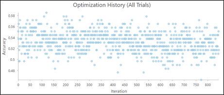
If you optimize the hyperparameters, the Output Parameter Tuning Table parameter is available. The Output Parameter Tuning Table value lists every set of hyperparameters values that have been searched and includes the following charts:
- Optimization History (All Trails)—A chart that visualizes the optimization history.
- Model Parameter Performance—A chart that helps evaluate the contribution of each hyperparameter to the model performance.
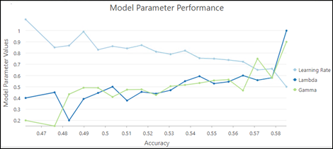
In this example, higher lambda and gamma values lead to higher model accuracy, while lower learning rates lead to a higher model accuracy.
Best practices
The following are best practices when using this tool:
- The tool may perform poorly when trying to predict with explanatory variables that are outside of the range of the explanatory variables used to train the model. Forest-based and boosted models do not extrapolate; they can only classify or predict to the value range on which the model was trained. If you use explanatory variables with a much higher or lower range than the original training dataset to make predictions, the model will estimate the value to be around the highest or lowest value in the original dataset.
- To improve performance when extracting values from the Explanatory Training Rasters value and calculating distances using the Explanatory Training Distance Features parameter, consider training the model on 100 percent of the data without excluding data for validation, and choose to create the Output Trained Features value. The next time you run the tool, use the Output Trained Features value as your Input Training Features parameter value and use all the extracted values and distances as Explanatory Training Variables value instead of extracting them each time you train the model. If you choose to do this, set the Number of Trees, Maximum Tree Depth and Number of Randomly Sampled Variables parameter values to 1 to create a very small placeholder tree to quickly prepare your data for analysis.
- For performance reasons, the Explanatory Training Distance Features parameter is not available when the Prediction Type parameter value is Predict to raster. To include distances to features as explanatory variables, calculate distance rasters using the Distance Accumulation tool, and include the distance rasters in the Explanatory Training Rasters parameter.
- Although the default Number of Trees parameter value is 100, this number is not data driven. The number of trees needed increases with the complexity of relationships between the explanatory variables, size of the dataset, and the variable to predict, in addition to the variation of these variables.
- Increase the number of trees in the forest and keep track of the OOB or classification error. It is recommended that you increase the Number of Trees value at least three times, up to at least 500 trees, to best evaluate model performance.
- Tool run time is highly sensitive to the number of variables used per tree. Using a small number of variables per tree decreases the chances of overfitting. However, be sure to use many trees if you're using a small number of variables per tree to improve model performance.
When using the gradient boosted model type, tool run time is highly affected by the Maximum Number of Bins for Searching Splits parameter value. The default value for the Number of Bins parameter is 0, which corresponds to the use of a greedy algorithm. This algorithm will create a candidate split at every data point which may cause a long run time. Therefore, when the size of the data is large or if there are many search points in the optimization, consider using a reasonable value for the Number of Bins of Searching Splits parameter.
- To create a model that does not change with every run, a seed can be set in the Random Number Generator environment setting. There will still be randomness in the model, but that randomness will be consistent between runs.
- Variable importance is a diagnostic that helps you understand which variables are driving the results of the model. It does not measure how well the model is predicting. A best practice is to use all the data for training by setting Training Data Excluded for Validation (%) value to 0 and exploring the variable importance box plot. Next, modify other parameters, such as Number of Trees or Maximum Tree Depth, and explore the box plots until you have a stable model. Once a stable model with regard to variable importance is trained, you can increase the Training Data Excluded for Validation (%) value to determine the accuracy of your model. If the model specified is Forest-based model, explore the OOB errors in the diagnostic messages to determine the accuracy of your model. Once you have a model that has stable variable importance and is accurate, you can set the Number of Runs for Validation value to 1 and obtain a single bar chart that depicts the final variable importance of your model.
References
Breiman, Leo. (1996). "Out-Of-Bag Estimation." Abstract.
Breiman, L. (1996). "Bagging predictors." Machine learning 24 (2): 123–140.
Breiman, Leo. (2001). "Random Forests." Machine Learning 45 (1): 5-32. https://doi.org/10.1023/A:1010933404324.
Breiman, L., J.H. Friedman, R.A. Olshen, and C.J. Stone. (2017). Classification and regression trees. New York: Routledge. Chapter 4.
Chen, T., and Guestrin, C. (2016). "XGBoost: A Scalable Tree Boosting System." In Proceedings of the 22nd ACM SIGKDD Conference on Knowledge Discovery and Data Mining. 785-794.
Dietterich, T. G. (2000, June). "Ensemble methods in machine learning." In International workshop on multiple classifier systems,. 1–15. Springer, Berlin, Heidelberg.
Gini, C. 1912 1955. Variabilità e mutabilità. Reprinted in Memorie di metodologica statistica (eds. E. Pizetti and T. Salvemini). Rome: Libreria Eredi Virgilio Veschi.
Grömping, U. (2009). "Variable importance assessment in regression: linear regression versus random forest." The American Statistician 63 (4): 308–319.
Ho, T. K. (1995, August). "Random decision forests." In Document analysis and recognition, 1995., proceedings of the third international conference on Document Analysis and Recognition Vol. 1: 278-282. IEEE.
James, G., D. Witten, T. Hastie, and R. Tibshirani. (2013). An introduction to statistical learning Vol. 112. New York: springer.
LeBlanc, M. and R. Tibshirani. (1996). "Combining estimates in regression and classification." Journal of the American Statistical Association 91 (436): 1641–1650.
Loh, W. Y. and Y. S. Shih. (1997). "Split selection methods for classification trees." Statistica sinica, 815–840.
Meinshausen, Nicolai. "Quantile regression forests." Journal of Machine Learning Research 7. Jun (2006): 983-999.
Nadeau, C. and Y. Bengio. (2000). "Inference for the generalization error." In Advances in neural information processing systems, 307-313.
Strobl, C., A. L. Boulesteix, T. Kneib, T. Augustin, and A. Zeileis. (2008). "Conditional variable importance for random forests." BMC bioinformatics 9 (1): 307.
Zhou, Z. H. (2012). "Ensemble methods: foundations and algorithms." CRC press.

