Geographically Weighted Regression (GWR) (Spatial Statistics)

Summary

Performs Geographically Weighted Regression (GWR), which is a local form of linear regression that is used to model spatially varying relationships.

Note:

This tool was added at ArcGIS Pro 2.3 to replace the similar but now deprecated Geographically Weighted Regression (GWR) tool. This new tool includes improvements to the method developed over the past several years and supports additional models.

Learn more about how Geographically Weighted Regression (GWR) works

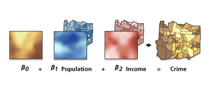
Illustration

Geographically Weighted Regression
GWR is a local regression model. Coefficients are allowed to vary across space.

Usage

  • This tool performs Geographically Weighted Regression (GWR), a local form of regression used to model spatially varying relationships. The GWR tool provides a local model of the variable or process you are trying to understand or predict by fitting a regression equation to every feature in the dataset. The Geographically Weighted Regression (GWR) tool constructs these separate equations by incorporating the dependent and explanatory variables of features within the neighborhood of each target feature. The shape and extent of each neighborhood analyzed is based on the input for the Neighborhood Type and Neighborhood Selection Method parameters with one restriction: when the number of neighboring features will exceed 1000, only the closest 1000 are incorporated into each local equation.

  • Apply the GWR tool to datasets with several hundred features for best results. It is not an appropriate method for small datasets. The tool does not work with multipoint data.

  • Use the Input Features parameter with a field representing the phenomena you are modeling (the Dependent Variable) and one or more fields representing the Explanatory Variable(s). These fields must be numeric and have a range of values. Features that contain missing values in the dependent or explanatory variable will be excluded from the analysis; however, you can use the Fill Missing Values tool to complete the dataset before running the Geographically Weighted Regression (GWR) tool.

  • Note:

    The Geographically Weighted Regression (GWR) tool produces a variety of outputs. A summary of the GWR model is available as a message at the bottom of the Geoprocessing pane during tool execution. You can access the message by hovering over the progress bar, clicking the pop-out button, or expanding the messages section in the Geoprocessing pane. You can also access the messages of a previously run Geographically Weighted Regression (GWR) tool via the geoprocessing history.

    The GWR tool also produces Output Features and adds fields reporting local diagnostic values. The Output Features and associated charts are automatically added to the table of contents with a hot/cold rendering scheme applied to model residuals. A full explanation of each output and chart is provided in How Geographically Weighted Regression works.

  • The Model Type specified depends on the data you are modeling. It is important to use the correct model for your analysis to obtain accurate results of your regression analysis.

  • It is recommended that you use projected data. This is especially important when distance is a component of the analysis, as it is for GWR when you select Distance band for the Neighborhood Type parameter. It is recommended that your data is projected using a projected coordinate system (rather than a geographic coordinate system).

  • Some of the Geographically Weighted Regression (GWR) tool computations take advantage of multiple CPUs to increase performance and will automatically use up to eight threads/CPUs for processing.

  • It is common practice to explore your data globally using the Generalized Linear Regression tool prior to exploring your data locally using the GWR tool.

  • The Dependent Variable and Explanatory Variable(s) parameters should be numeric fields containing a variety of values. There should be variation in these values both globally and locally. For this reason, do not use dummy explanatory variables to represent different spatial regimes in your GWR model (such as assigning a value of 1 to census tracts outside the urban core, while all others are assigned a value of 0). Because the GWR tool allows explanatory variable coefficients to vary, these spatial regime explanatory variables are unnecessary, and if included, will create problems with local multicollinearity.

  • In global regression models, such as Generalized Linear Regression, results are unreliable when two or more variables exhibit multicollinearity (when two or more variables are redundant or together tell the same story). The GWR tool builds a local regression equation for each feature in the dataset. When the values for a particular explanatory variable cluster spatially, it is likely that there are problems with local multicollinearity. The condition number field (COND) in the output feature class indicates when results are unstable due to local multicollinearity. As a general rule, be skeptical of results for features with a condition number greater than 30, equal to Null or, for shapefiles, equal to -1.7976931348623158e+308. The condition number is scale-adjusted to correct for the number of explanatory variables in the model. This allows direct comparison of the condition number between models using different numbers of explanatory variables.

  • Use caution when including nominal or categorical data in a GWR model. Where categories cluster spatially, there is risk of encountering local multicollinearity issues. The condition number included in the GWR output indicates when local collinearity is a problem (a condition number less than 0, greater than 30, or set to Null). Results in the presence of local multicollinearity are unstable.

  • To better understand regional variation among the coefficients of your explanatory variables, examine the optional raster coefficient surfaces created by the GWR tool. These raster surfaces are created in the Coefficient Raster Workspace parameter, under Additional Options, if specified. For polygon data, you can use graduated color or cold-to-hot rendering on each coefficient field in the Output Features to examine changes across your study area.

  • You can use the GWR tool for prediction by supplying Predictions Locations (often this feature class is the same as Input Features), matching the explanatory variables and specifying Output Predicted Features. If the Explanatory Variables to Match fields from Input Features match the Fields From Prediction Locations fields, they will automatically populate. If not, specify the correct fields.

  • A regression model is incorrectly specified if it is missing a key explanatory variable. Statistically significant spatial autocorrelation of the regression residuals or unexpected spatial variation among the coefficients of one or more explanatory variables suggests that your model is incorrectly specified. You should make every effort (through GLR residual analysis and GWR coefficient variation analysis, for example) to discover these key missing variables so they can be included in the model.

  • Always question whether it makes sense for an explanatory variable to be nonstationary. For example, suppose you are modeling the density of a particular plant species as a function of several variables including ASPECT. If you find that the coefficient for the ASPECT variable changes across the study area, you are likely seeing evidence of a key missing explanatory variable (perhaps prevalence of competing vegetation, for example). You should make every effort to include all key explanatory variables in your regression model.

  • When the result of a computation is infinity or undefined, the result for nonshapefiles will be Null; for shapefiles, the result will be -DBL_MAX = -1.7976931348623158e+308.

    Caution:

    When using shapefiles, keep in mind that they cannot store null values. Tools or other procedures that create shapefiles from nonshapefile inputs may, consequently, store null values as zero or as some very small negative number (-DBL_MAX = -1.7976931348623158e+308). This can lead to unexpected results. For more information see Geoprocessing considerations for shapefile output.

  • There are three options for the Neighborhood Selection Method parameter. When you select Golden search, the tool will find the best values for the Distance Band or Number of Neighbors parameter using the golden section search method. The Manual intervals option will test neighborhoods in increments between the distances specified. In either case, the neighborhood size used is the one that minimizes the Akaike information criterion (AICc) value. Problems with local multicollinearity, however, will prevent both of these methods from resolving an optimal distance band or number of neighbors. If you receive an error or run into severe model design problems, you can try specifying a particular distance or neighborhood count using the User defined option. Then examine the condition numbers in the output feature class to see which features are associated with local collinearity problems.

  • Severe model design issues, or errors indicating local equations do not include enough neighbors, often indicate a problem with global or local multicollinearity. To determine where the problem is, run a global model using Generalized Linear Regression and examine the VIF value for each explanatory variable. If some of the VIF values are large (above 7.5, for example), global multicollinearity is preventing GWR from solving. More likely, however, local multicollinearity is the problem. Try creating a thematic map for each explanatory variable. If the map reveals spatial clustering of identical values, consider removing those variables from the model or combining them with other explanatory variables to increase value variation. If, for example, you are modeling home values and have variables for bedrooms and bathrooms, you can combine these to increase value variation or to represent them as bathroom/bedroom square footage. Avoid using spatial regime dummy variables, spatially clustering categorical or nominal variables, or variables with very few possible values when constructing GWR models.

  • Geographically Weighted Regression is a linear model subject to the same requirements as Generalized Linear Regression . Review the diagnostics explained in How Geographically Weighted Regression works to ensure your GWR model is properly specified. The How regression models go bad section in the Regression analysis basics topic also includes information for ensuring your model is accurate.

Parameters

LabelExplanationData Type
Input Features

The feature class containing the dependent and explanatory variables.

Feature Layer
Dependent Variable

The numeric field containing the observed values that will be modeled.

Field
Model Type

Specifies the type of data that will be modeled.

  • Continuous (Gaussian) The Dependent Variable value is continuous. The Gaussian model will be used, and the tool will perform ordinary least squares regression.
  • Binary (Logistic) The Dependent Variable value represents presence or absence. This can be either conventional 1s and 0s or continuous data that has been coded based on a threshold value. The Logistic regression model will be used.
  • Count (Poisson)The Dependent Variable value is discrete and represents events, such as crime counts, disease incidents, or traffic accidents. The Poisson regression model will be used.
String
Explanatory Variable(s)

A list of fields representing independent explanatory variables in the regression model.

Field
Output Features

The new feature class containing the dependent variable estimates and residuals.

Feature Class
Neighborhood Type

Specifies whether the neighborhood used is constructed as a fixed distance or allowed to vary in spatial extent depending on the density of the features.

  • Number of neighbors The neighborhood size is a function of a specified number of neighbors included in calculations for each feature. Where features are dense, the spatial extent of the neighborhood is smaller; where features are sparse, the spatial extent of the neighborhood is larger.
  • Distance bandThe neighborhood size is a constant or fixed distance for each feature.
String
Neighborhood Selection Method

Specifies how the neighborhood size will be determined. The neighborhood selected with the Golden search and Manual intervals options is based on minimizing the AICc value.

  • Golden searchThe tool will identify an optimal distance or number of neighbors based on the characteristics of the data using the golden section search method.
  • Manual intervals The neighborhoods tested will be defined by the values specified in the Minimum Number of Neighbors and Number of Neighbors Increment parameters when Number of neighbors is chosen for the Neighborhood Type parameter, or the Minimum Search Distance and Search Distance Increment parameters when Distance band is chosen for the Neighborhood Type parameter, as well as the Number of Increments parameter.
  • User defined The neighborhood size will be specified by either the Number of Neighbors or Distance Band parameter.
String
Minimum Number of Neighbors
(Optional)

The minimum number of neighbors each feature will include in its calculations. It is recommended that you use at least 30 neighbors.

Long
Maximum Number of Neighbors
(Optional)

The maximum number of neighbors (up to 1000) each feature will include in its calculations.

Long
Minimum Search Distance
(Optional)

The minimum neighborhood search distance. It is recommended that you use a distance at which each feature has at least 30 neighbors.

Linear Unit
Maximum Search Distance
(Optional)

The maximum neighborhood search distance. If a distance results in features with more than 1000 neighbors, the tool will use the first 1000 in calculations for the target feature.

Linear Unit
Number of Neighbors Increment
(Optional)

The number of neighbors by which manual intervals will increase for each neighborhood test.

Long
Search Distance Increment
(Optional)

The distance by which manual intervals will increase for each neighborhood test.

Linear Unit
Number of Increments
(Optional)

The number of neighborhood sizes to test starting with the Minimum Number of Neighbors or Minimum Search Distance parameter.

Long
Number of Neighbors
(Optional)

The closest number of neighbors (up to 1000) to consider for each feature. The number must be an integer between 2 and 1000.

Long
Distance Band
(Optional)

The spatial extent of the neighborhood.

Linear Unit
Prediction Locations
(Optional)

A feature class containing features representing locations where estimates will be computed. Each feature in this dataset should contain values for all the explanatory variables specified. The dependent variable for these features will be estimated using the model calibrated for the input feature class data. To be predicted, these feature locations should be within the same study area as the Input Features or be close (within the extent plus 15 percent).

Feature Layer
Explanatory Variables to Match
(Optional)

The explanatory variables from the Prediction Locations parameter that match corresponding explanatory variables from the Input Feature Class parameter.

Value Table
Output Predicted Features
(Optional)

The output feature class that will receive dependent variable estimates for each Prediction Location.

Feature Class
Robust Prediction
(Optional)

Specifies the features that will be used in prediction calculations.

  • Checked—Features with values more than three standard deviations from the mean (value outliers) and features with weights of 0 (spatial outliers) will be excluded from prediction calculations but will receive predictions in the output feature class. This is the default.
  • Unchecked—All features will be used in prediction calculations.
Boolean
Local Weighting Scheme
(Optional)

Specifies the kernel type that will be used to provide the spatial weighting in the model. The kernel defines how each feature is related to other features within its neighborhood.

  • BisquareA weight of 0 will be assigned to any feature outside the neighborhood specified. This is the default.
  • GaussianAll features will receive weights, but weights become exponentially smaller the farther away they are from the target feature.
String
Coefficient Raster Workspace
(Optional)

The workspace where the coefficient rasters will be created. When this workspace is provided, rasters are created for the intercept and every explanatory variable.

Workspace

Derived Output

LabelExplanationData Type
Coefficient Raster Layers

The output coefficient rasters.

Raster Layer

arcpy.stats.GWR(in_features, dependent_variable, model_type, explanatory_variables, output_features, neighborhood_type, neighborhood_selection_method, {minimum_number_of_neighbors}, {maximum_number_of_neighbors}, {minimum_search_distance}, {maximum_search_distance}, {number_of_neighbors_increment}, {search_distance_increment}, {number_of_increments}, {number_of_neighbors}, {distance_band}, {prediction_locations}, {explanatory_variables_to_match}, {output_predicted_features}, {robust_prediction}, {local_weighting_scheme}, {coefficient_raster_workspace})
NameExplanationData Type
in_features

The feature class containing the dependent and explanatory variables.

Feature Layer
dependent_variable

The numeric field containing the observed values that will be modeled.

Field
model_type

Specifies the type of data that will be modeled.

  • CONTINUOUS The dependent_variable value is continuous. The Gaussian model will be used, and the tool will perform ordinary least squares regression.
  • BINARY The dependent_variable value represents presence or absence. This can be either conventional 1s and 0s or continuous data that has been coded based on a threshold value. The Logistic regression model will be used.
  • COUNTThe dependent_variable value is discrete and represents events, such as crime counts, disease incidents, or traffic accidents. The Poisson regression model will be used.
String
explanatory_variables
[explanatory_variables,...]

A list of fields representing independent explanatory variables in the regression model.

Field
output_features

The new feature class containing the dependent variable estimates and residuals.

Feature Class
neighborhood_type

Specifies whether the neighborhood used is constructed as a fixed distance or allowed to vary in spatial extent depending on the density of the features.

  • NUMBER_OF_NEIGHBORS The neighborhood size is a function of a specified number of neighbors included in calculations for each feature. Where features are dense, the spatial extent of the neighborhood is smaller; where features are sparse, the spatial extent of the neighborhood is larger.
  • DISTANCE_BANDThe neighborhood size is a constant or fixed distance for each feature.
String
neighborhood_selection_method

Specifies how the neighborhood size will be determined. The neighborhood selected with the GOLDEN_SEARCH and MANUAL_INTERVALS options is based on minimizing the AICc value.

  • GOLDEN_SEARCHThe tool will identify an optimal distance or number of neighbors based on the characteristics of the data using the golden section search method.
  • MANUAL_INTERVALS The neighborhoods tested will be defined by the values specified in the minimum_number_of_neighbors and number_of_neighbors_increment parameters when NUMBER_OF_NEIGHBORS is chosen for the neighborhood_type parameter, or the minimum_search_distance and search_distance_increment parameters when DISTANCE_BAND is chosen for the neighborhood_type parameter, as well as the number_of_increments parameter.
  • USER_DEFINED The neighborhood size will be specified by either the number_of_neighbors or distance_band parameter.
String
minimum_number_of_neighbors
(Optional)

The minimum number of neighbors each feature will include in its calculations. It is recommended that you use at least 30 neighbors.

Long
maximum_number_of_neighbors
(Optional)

The maximum number of neighbors (up to 1000) each feature will include in its calculations.

Long
minimum_search_distance
(Optional)

The minimum neighborhood search distance. It is recommended that you use a distance at which each feature has at least 30 neighbors.

Linear Unit
maximum_search_distance
(Optional)

The maximum neighborhood search distance. If a distance results in features with more than 1000 neighbors, the tool will use the first 1000 in calculations for the target feature.

Linear Unit
number_of_neighbors_increment
(Optional)

The number of neighbors by which manual intervals will increase for each neighborhood test.

Long
search_distance_increment
(Optional)

The distance by which manual intervals will increase for each neighborhood test.

Linear Unit
number_of_increments
(Optional)

The number of neighborhood sizes to test starting with the minimum_number_of_neighbors or minimum_search_distance parameter.

Long
number_of_neighbors
(Optional)

The closest number of neighbors (up to 1000) to consider for each feature. The number must be an integer between 2 and 1000.

Long
distance_band
(Optional)

The spatial extent of the neighborhood.

Linear Unit
prediction_locations
(Optional)

A feature class containing features representing locations where estimates will be computed. Each feature in this dataset should contain values for all the explanatory variables specified. The dependent variable for these features will be estimated using the model calibrated for the input feature class data. To be predicted, these feature locations should be within the same study area as the in_features or be close (within the extent plus 15 percent).

A feature class containing features representing locations where estimates will be computed. Each feature in this dataset should contain values for all the explanatory variables specified. The dependent variable for these features will be estimated using the model calibrated for the input feature class data. To be predicted, these feature locations should be within the same study area as the Input Features or be close (within the extent plus 15 percent).

Feature Layer
explanatory_variables_to_match
[explanatory_variables_to_match,...]
(Optional)

The explanatory variables from the prediction_locations parameter that match corresponding explanatory variables from the in_features parameter. [["LandCover2000", "LandCover2010"], ["Income", "PerCapitaIncome"]] are examples.

Value Table
output_predicted_features
(Optional)

The output feature class that will receive dependent variable estimates for each prediction_location.

Feature Class
robust_prediction
(Optional)

Specifies the features that will be used in prediction calculations.

  • ROBUSTFeatures with values more than three standard deviations from the mean (value outliers) and features with weights of 0 (spatial outliers) will be excluded from prediction calculations but will receive predictions in the output feature class. This is the default.
  • NON_ROBUSTAll features will be used in prediction calculations
Boolean
local_weighting_scheme
(Optional)

Specifies the kernel type that will be used to provide the spatial weighting in the model. The kernel defines how each feature is related to other features within its neighborhood.

  • BISQUAREA weight of 0 will be assigned to any feature outside the neighborhood specified. This is the default.
  • GAUSSIANAll features will receive weights, but weights become exponentially smaller the farther away they are from the target feature.
String
coefficient_raster_workspace
(Optional)

The workspace where the coefficient rasters will be created. When this workspace is provided, rasters are created for the intercept and every explanatory variable.

Workspace

Derived Output

NameExplanationData Type
coefficient_raster_layers

The output coefficient rasters.

Raster Layer

Code sample

GWR example 1 (Python window)

The following Python window script demonstrates how to use the GWR tool.

import arcpy
arcpy.env.workspace = r"c:\data\project_data.gdb”
arcpy.stats.GWR("US_Counties", "Diabetes_Percent", "CONTINUOUS", 
     "Inactivity_Percent;Obesity_Percent", "out_features", 
     "NUMBER_OF_NEIGHBORS", "GOLDEN_SEARCH", None, None, None, 
     None, None, None, None, None, None, None, None, None, "ROBUST", 
     "BISQUARE")
GWR example 2 (stand-alone script)

The following stand-alone Python script demonstrates how to use the GWR tool.

# Linear regression using a count model to predict the number of crimes.
# The depend variable (total number of crimes) is predicted using total
# population, the median age of housing, and average household income.
 
import arcpy

# Set the current workspace (to avoid having to specify the full path to
# the feature classes each time)

arcpy.env.workspace = r"c:\data\project_data.gdb"

arcpy.stats.GWR("crime_counts", "total crimes", "COUNT", "YRBLT;TOTPOP;AVGHINC", 
     "out_features", "NUMBER_OF_NEIGHBORS", "GOLDEN_SEARCH", 30, None, None, None, 
     None, None, None, None, None, "prediction_locations", 
     "YRBLT YRBLT;TOTPOP TOTPOP;AVGHINC AVGHINC", "predicted_counts", 
     "NON_ROBUST", "BISQUARE", r"c:\data\out_rasters")

Environments

Output Coordinate System

Feature geometry is projected to the output coordinate system after analysis is complete.

Licensing information

  • Basic: Limited
  • Standard: Limited
  • Advanced: Yes

Related topics