How Derive Continuous Flow works

Available with Spatial Analyst license.

Understanding how water moves through the landscape after it falls in the form of precipitation is fundamental for many applications. Digital elevation models (DEMs) are the foundational dataset for modeling surface flow. However, this data is not a perfect representation—there are often small elevation errors or misrepresentations of landscape features, which may impact flow.

Therefore, you must preprocess the input DEM before determining water flow direction. Hydroconditioning refers to the exercise of modifying the input DEM elevation values to ensure continuous surface flow representative of actual surface flow. Hydroconditioning is necessary to address instances in which DEM limitations disrupt the flow network, for example, spurious elevation can act as sinks that artificially accumulate and terminate flow, making it impossible to determine the direction of flow outward from the sink cells. Bridges, dams, and culverts that are not included in the surface model can also create erroneous flow direction and accumulation outputs.

The Derive Continuous Flow tool addresses erroneous flow direction and accumulation outputs, not by modifying the input DEM data, but through the application of the least-cost path algorithm. The least-cost path algorithm involves a minimization of elevation difference moving uphill across the input surface raster. In other words, on a cell-by-cell basis, an optimization step is required to identify the minimum upslope neighbor. Additionally, special rules for sink cells and NoData cells are also applied. Sink or depression cells can be individual cells or a group of cells whose neighbors have a higher elevation value than that of the processing cell or group of cells. NoData cells are considered places of unknown information and are not used in processing.

This tool uses a DEM surface as input and creates a raster showing the direction and accumulation of flow at each cell.

If the input surface raster contains real sinks or depression areas, they should be specified using the Input raster or feature depressions data parameter. If a raster dataset is specified, cells in the input raster with data will be considered valid depression cells. If a feature dataset is specified, the features are rasterized to the same resolution as the input surface data, and the resulting raster is used to specify valid depression cells.

The tool provides two methods for determining flow direction using the Flow direction type parameter: The D8 method models flow direction from each cell to its steepest downslope neighbor and is limited to a single direction (Jenson and Domingue, 1988). The MFD (Multiple Flow Direction) method allows for flow partitioning across all downslope neighbors using an approach that adapts the flow partitioning exponent depending on local terrain conditions (Qin et al., 2007).

When Input accumulation weight raster is specified, a weight is applied to each cell when deriving accumulation.

Calculate flow direction and flow accumulation

In the Derive Continuous Flow algorithm, there are two basic steps in the least-cost path approach applied to flow routing. First, valid outlets are set. Valid outlets are cells where water can flow into but not outwards. By default, outlet cells are cells at the edge of the input surface raster. If Input raster or feature depressions data is specified, cells in the input raster or feature dataset will also be marked as valid outlets from the start of the algorithm. The second step is to traverse the input surface raster and derive flow direction and flow accumulation at each cell by processing cells in order from lowest elevation to highest elevation. These two principles allow movement from the current cell to the next higher cell in the direction of the least steep uphill slope (Metz et al., 2011; Ehlschlaeger, 1989).

The following diagram shows the general logic followed. Special cases such as depression (sink) cells not explicitly specified as depressions through the Input raster or depressions data parameter and NoData are explained in the Process unknown depression cells and NoData cells in the input surface raster sections, respectively.

Figure 1. The least-cost path algorithm for determining flow routing and accumulation, as described in Metz et al., 2011; Ehlschlaeger, 1989, is shown.

Derive Continuous Flow logic

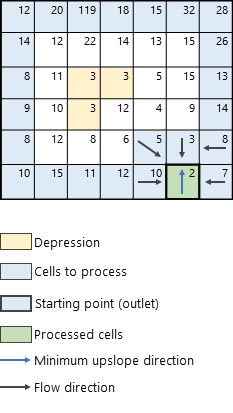
In this section, you will step through an example of how the Derive Continuous Flow tool processes elevation data and determines flow direction and accumulation cell-by-cell. This example demonstrates the process in the presence of a depression that was not included in the optional Input raster or feature depressions data parameter (see Figure 2).

Figure 2. An example of synthetic elevation data with cell size equal to 1 is shown. This example has a depression around the middle area of the surface raster, shown in yellow, which was not specified in the Input raster or features depressions data parameter.

First, outlets are identified. These correspond to cells at the edge of the map (colored in blue in Figure 3).

Figure 3. Outlet candidate cells identified as potential outlets in step 1 are shown.

Once outlet cells have been identified (blue colored cells), the algorithm proceeds to find the cell with the lowest elevation from which the search will start. In this example, the lowest cell (with elevation 2) is highlighted with a thick black border in Figure 4.

Figure 4. In step 2, the starting point is identified by sorting potential outlet cells by elevation and choosing the one with the lowest elevation, highlighted with a thick black border.

The next step is to identify the neighbors of the processing cell (colored in green) whose elevation value is greater than that of the processing cell. These neighbors are added to the possible cells that can be processed next, shown in Figure 5. The next cell to process is determined by finding the lowest elevation uphill neighbor (in this example, the cell with elevation value 3) that corresponds to the minimum upslope direction (the blue arrow in Figure 5). The direction of flow and accumulation for the neighboring uphill cells are computed sequentially for the processing cell. Flow direction is determined using the method specified in the Flow direction type parameter. There are two available methods to determine flow direction, D8 and MFD. For a detailed explanation of these two methods, see the Flow direction methods section below.

Figure 5. In step 3, the neighboring cells of the current processing cell have been identified. Cells highlighted in blue are cells that can potentially be processed next. Black arrows correspond to flow direction, and blue arrows correspond to the path to follow for processing.

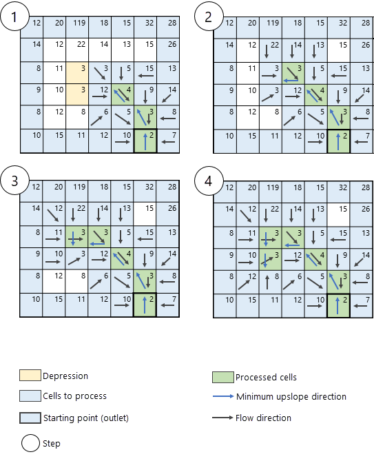
The algorithm continues in the same manner, identifying neighboring cells to the current processing cell following the direction of the minimum upslope. The next iteration of the algorithm is shown in Figure 6.

Figure 6. The next iteration is shown. As in Figure 5, cells highlighted in blue are cells that can potentially be processed next. The next cell to process in this diagram is 3, colored green. Black arrows correspond to flow direction, and blue arrows correspond to the least-cost path direction.

Process unknown depression cells

Depression (or sink) cells can be individual cells or a group of cells whose neighbors have a higher elevation value than that of the processing cell or group of cells. If these are not included in the Input raster or feature depressions data parameter, they will be unknown depression cells to the tool. Under this scenario, if an unknown depression cell or group of cells are encountered, the path follows the steepest descent (instead of following the lowest uphill neighboring cell) until reaching the bottom of the depression, setting flow direction and accumulation along the depression path. This process is shown in Figure 7.

Figure 7. The sequence of processing each cell within the depression, from left to right, is shown. Flow direction and accumulation is determined as each cell within the depression is processed. Processing direction through the depression is toward the steepest descent, instead of following the lowest uphill neighboring cell.

NoData cells in the input surface raster

NoData cells in the input surface raster are cells whose value is not known. These cells can exist in the surface raster and can be encountered during the Derive Continuous Flow algorithm. If this is the case, they are not processed and the algorithm passes around them, as shown in Figure 8.

Figure 8. NoData cells within the input surface raster are ignored by the Derive Continuous Flow tool. Exterior NoData cells push the input surface raster boundary to the neighbors with valid data values. The rest of the calculations to determine flow direction and accumulation remain the same.

Flow direction methods

In the D8 method, the direction of flow is determined by the direction of steepest descent, or maximum drop, from each cell (Jenson and Domingue, 1988). This is calculated as follows:

maximum_drop = change_in_z-value/distance

Distance is calculated between cell centers. For corner-neighboring cells, the algorithm verifies that the maximum drop toward the current processing cell is the maximum; otherwise, flow direction will be set toward the cell with the maximum drop of the given corner-neighboring cell. If a cell has the same change in z-value in multiple directions, D8 flow direction is ambiguous, and the value will be the sum of the possible directions.

When a direction of steepest descent is found, the output cell is coded with the value representing that direction.

In the MFD method, flow is partitioned across all downslope neighbors (Qin et al., 2007). The amount of flow each downslope neighbor receives is estimated as a function of the maximum slope gradient, which allows for local terrain conditions. The expression for estimating MFD is as follows:

Where:

• d_i = Portion of flow from each cell that flow into cell i
• f (e) = Exponent that adapts to local terrain conditions and it is given by

  

• β = Downslope angle (in radians)
• n = number of cells that flow into cell i
• L_i, L_j = Adjusted factor to account for distance between processing cell and orthogonal and diagonal cells
• κ = Maximum drop across cells that flow into cell i

Once flow direction and accumulation have been determined, as well as the direction of the least-cost path, the processing cell is marked as processed, and the next cell in the queue is analyzed. The algorithm proceeds in this manner until all cells in the input surface raster have been processed. In other words, flow direction and accumulation have been determined for all cells.

References

Ehlschlaeger, C. R. 1989. "Using the AT Search Algorithm to Develop Hydrologic Models from Digital Elevation Data." International Geographic Information Systems (IGIS) Symposium 89: 275-281.

Jenson, S. K., and Domingue, J. O. 1988. "Extracting Topographic Structure from Digital Elevation Data for Geographic Information System Analysis." Photogrammetric Engineering and Remote Sensing 54 (11): 1593–1600.

Metz, M., Mitasova, H., & Harmon, R. S. 2011. "Efficient extraction of drainage networks from massive, radar-based elevation models with least cost path search." Hydrology and Earth System Sciences 15(2): 667-678.

Qin, C., Zhu, A. X., Pei, T., Li, B., Zhou, C., & Yang, L. 2007. "An adaptive approach to selecting a flow partition exponent for a multiple flow direction algorithm." International Journal of Geographical Information Science 21(4): 443-458.