How Multiscale Surface Percentile works

Available with Spatial Analyst license.

Analyzing topography and other surfaces is an important part of many disciplines, ranging from hydrology to ecology. The results of such analyses often depend on the spatial resolution of the data or calculations for a particular topographic characteristic. This dependency has caused a rise in multiscale analysis approaches, analyses where calculations are done for multiple spatial resolutions. These multiscale approaches can be used to find the optimum scale to characterize a topography and measure how parameters respond to changes in scale.

The Multiscale Surface Percentile tool calculates the most extreme percentile across a range of spatial scales (neighborhoods ranging in size). The percentile furthest from 50 (such as values closer to 0 or 100) is considered the most extreme value for a given cell. The outputs of this tool identify this percentile for a cell and the scale at which it was found.

The outputs can be used to interpret feature on an input surface raster and their associated scales. The example below shows the results of two different scales for the same surface. The first image (left) used a scale of 29 cells by 29 cells while the second image (right) used a scale of 49 cells by 49 cells. Here the smaller scale is more sensitive to local variation in the landscape and captures smaller surface features. On the other hand, the larger scale shows less detail by only capturing larger surface features.

Percentile output at the same extent is shown for two different scales, a small scale (second graphic) and a larger scale (third graphic).

How the most extreme percentile value is calculated

The following steps provide an overview of the internal processes used by the tool:

1. The scales for analysis are defined using the Minimum Neighborhood Distance, Maximum Neighborhood Distance, Base Distance Increment, and Nonlinearity Factor parameters. The units of these parameters are controlled by the Distance Units parameter.
2. For each cell, percentile is calculated at each identified scale.
3. The calculated percentiles are compared across scales. The percentile furthest from 50 is considered the most extreme percentile for a given cell.

Each of these steps are explained in more detail in the sections below.

How the scales to analyze are identified

The scales for analysis are determined using the optional parameters in the Multiscale Surface Percentile tool. The Minimum Neighborhood Distance and Maximum Neighborhood Distance parameters set the minimum and maximum scales for analysis. The Base Distance Increment and Nonlinearity Factor parameters control the increase in neighborhood distance between the minimum and maximum.

Each scale is represented as a neighborhood distance value. Analysis is performed for multiple neighborhood distances depending on the input parameter settings.

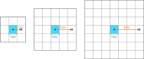
For a given target cell, the neighborhood distance is measured from the target cell center outward, creating a square of cells around the target cell. For example, a neighborhood distance of 30 meters for an input surface raster with a 10 meter cell size results in a neighborhood that is 7 cells by 7 cells, as shown in the figure below. This value, 30 meters, would be one of the scales for which the most extreme percentile is calculated.

The relationship between neighborhood distance (orange line) and the number in pixels of the moving window is shown. For a cell size of 10 meters, a neighborhood distance of 10 meters will use a 3 by 3 cell window (this is the default), a neighborhood distance of 20 meters will use a 5 by 5 cell window, and a neighborhood distance of 30 meters will use a 7 by 7 cell window.

The smallest allowed neighborhood distance is equal to the cell size of the input raster. This is a value of 1 cell, and creates a 3 by 3 neighborhood of cells. In the example above, this minimum is a neighborhood distance of 5 meters.

The neighborhood distance cannot be larger than the input surface raster.

If a neighborhood distance that does not result in an interval of the cell size is specified, the tool will round the distance up to the next interval of the cell size. For example, in the illustration above, if a neighborhood distance of 25 meters is specified, it will round up to the next interval of the cell size, which is 30 meters.

Calculations start with the Minimum Neighborhood Distance parameter value and then each subsequent neighborhood distance is calculated.

The expression for calculating the subsequent neighborhood distances to be used is as follows:

ni = no + [Δn × (i - no)]p

• Where:

  n_i = Neighborhood distance for step i

  n_o = Minimum neighborhood distance

  Δn = Base distance increment

  i = The step for which neighborhood distance is being calculated (where the 1st step has a value of 1 + n_o)

  p = Nonlinearity factor

Every new neighborhood distance identified is checked to determine if it is less than or equal to the Maximum Neighborhood Distance parameter value. If the new distance value is less than or equal to the maximum, neighborhood distance calculations continue. If the new value is greater than the maximum, all neighborhood distances have been identified and percentile calculations begin.

See the How percentile is calculated section below for more information on that portion of the analysis.

How the nonlinearity factor affects the neighborhood distances

The Nonlinearity Factor parameter controls the raster of increase in neighborhood distance. The default is a value of 1, which results in a linear increase in neighborhood distance. That means the increments between neighborhood distances will be equal to the Base Distance Increment parameter value.

When increasing the Nonlinearity Factor parameter value above 1, the increments between neighborhood distances will change after the first one. The first increment will be equal to the Base Distance Increment value, but all subsequent increments will progressively increase in size.

When the Nonlinearity Factor parameter value is set to values above 1, the increment in the distance between subsequent neighborhood distances after the first will progressively increase. Another consequence is that for the same minimum and maximum neighborhood values, a higher nonlinearity factor will result in fewer neighborhood distances overall.

The figure below illustrates the effect of three different settings of the Nonlinearity Factor parameter. In this example the settings are 1.0, 1.5, and 2.0. For each of these settings, the values for the other parameters are kept the same. The Minimum Neighborhood Distance parameter value is 1, the Maximum Neighborhood Distance value is 10, and the Base Distance Increment value is 1.

For the first increment, the neighborhood distance for all three settings of the nonlinearity factor is the same value, that being 2 cells. After this, the values for the neighborhood distance will start to vary. The increments will become progressively larger for a nonlinearity factor of 1.5, and more so for factor of 2.0.

When the Nonlinearity Factor parameter value is 1.0, there will be 9 increments in total, and each increment will be larger than the previous in a linear fashion. With a value of 1.5 for the factor, there will only be 4 increments, and 3 increments for a value of 2.0.

Increasing the Nonlinearity Factor above 1.0 causes increment sizes to progressively increase and therefore neighborhood distance increase faster. This also causes there to be less scales for the same Minimum Neighborhood Distance and Maximum Neighborhood Distance when a larger Nonlinearity Factor value is used.

The Nonlinearity Factor parameter allows you to customize the sampling density of scales. For elevation surface, elevation percentile is often more sensitive to neighborhood size at smaller scales and less sensitive at larger scales. Using a Nonlinearity Factor parameter value greater than 1.0 allows the scale sampling density to be higher for smaller scales and lower for larger scales. However, you may need to increase the Maximum Neighborhood Distance parameter value in these situations to get the desired number of inurements. For most situations, a value between 1.0 and 2.0 is used for the nonlinearity factor.

How percentile is calculated

Percentiles are a statistical measure that indicates the percentage of values in a dataset that fall below a given value. For example, the 80^th percentile is a value where you will find 80% of the values in the dataset are lower while the remaining 20% of values are higher.

For each neighborhood distance identified for calculation and each cell in the input surface raster, the Multiscale Surface Percentile tool calculates percentile. The most extreme percentile values are identified and recorded in the Output Percentile Raster parameter value. The scales at which those percentiles were found are recorded as the cell values in the Output Scale Raster parameter value.

The equation for calculating percentile at each cell is as follows:

Percentile = counti ∈C(zi < z0) × (100/nC)

• Where:

  C = The neighborhood identified for processing

  count_{i ∈C} = The number of cells in neighborhood C where (z_i<z₀) is true

  z_i = The value of cell i in neighborhood C

  z₀ = The value of neighborhood C's center cell

  n_C = The number of cells contained within neighborhood C

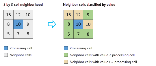
An example of this calculation is shown below with a 3 by 3 cell neighborhood.

The scale is 3 cells by 3 cells, and has 9 cells total. On the left, the value of the processing cell and the 8 surrounding cell values (grey) are identified. On the right, the cells whose values are less than the center cell (green) and values that are equal to or greater than the center cell (tan) are shown.

Applying the formula shown above to this example gives the following result:

Percentile = (Count of cell values less than center cell value) 
              * 100 / (Count of cells in neighborhood)
           = 5 * 100 / 9
           = 55.5556

This approach utilizes Huang et al. (1979)'s running-histogram filtering algorithm to bin percentile values as needed. Once a percentile value is found, the value is compared with the previously identified most extreme percentile. If the new value is more extreme, with a percentile further away from 50, the value is recorded for that location in the Output Percentile Raster parameter value. The scale value is recorded in the Output Scale Raster parameter value.

Use of a GPU

This tool can deliver increased performance if you have certain GPU hardware installed on your system. See GPU Processing with Spatial Analyst for details on how this capability is supported, how to configure it, and how to enable it.

References

Huang, Thomas S., G. Yang, and G. Tang. 1979. "A fast two-dimensional median filtering algorithm." IEEE Transactions on Acoustics, Speech, and Signal Processing Volume 27, Issue 1. pp.13–18. https://doi.org/10.1109/TASSP.1979.1163188

Newman, Daniel R., John B. Lindsay, and Jaclyn Mary Helen Cockburn. 2018. "Evaluating metrics of local topographic position for multiscale geomorphometric analysis." Geomorphology 312, 40–50. https://doi.org/10.1016/j.geomorph.2018.04.003