Spatial data often exhibits spatial autocorrelation, in which nearby observations have similar values. Ignoring this in regression models can lead to biased estimates and incorrect inferences.
The Spatial Autoregression tool is designed to address these challenges by fitting a spatial regression model that explicitly accounts for spatial dependence. The tool can perform either a traditional ordinary least squares regression or one of the following global spatial regression models: the spatial lag model, spatial error model, or spatial autoregressive combined model. You can specify which model the tool will use, or the tool can determine the most appropriate model by performing a series of diagnostic tests on the dependent and explanatory variables.
The objective of these regression models is to enable robust inference of regression models in the presence of spatial dependence. Using spatial regression models, you can be more confident in the estimates as well as provide estimates of the effects of space in your models.
Potential applications
The Spatial Autoregression tool can be used to account for spatial dependence in models in two primary ways.
First, the spatial lag model is valuable for analyzing spatial spillover effects, such as the following:
- Public health and epidemiology—Assess disease or virus spread while accounting for spatial dependence.
- Criminology—Understand how crime clusters and spreads geographically, incorporating neighborhood effects.
Second, the spatial error model can provide unbiased model estimates by accounting for spatial dependence in explanatory variables, such as the following:
- Socioeconomic analysis—Evaluate educational attainment while controlling for spatially correlated factors in explanatory variables.
- Housing prices—Control for unmeasured spatial factors affecting property values, providing clearer insight into key model variables.
Model types
The Spatial Autoregression tool can estimate three possible global spatial regression models, each of which account for spatial dependence in different ways. Ordinary least squares regression is performed when none of the three spatial regression models are determined to be suitable based on various diagnostics.
Spatial error model
The spatial error model (SEM) is designed to address situations in which there is spatial autocorrelation in the residuals of a regression model. For SEM, spatial dependence is viewed as a nuisance parameter. A nuisance parameter is one that must be accounted for in order to ensure that appropriate inferences are made. The SEM model is defined by the following formula:

It is similar to the ordinary least squares regression formula, in which a dependent variable (y) is predicted by a set of explanatory variable (x) and coefficients (β). However, the residual term (u) is modeled by a different regression equation. This second regression predicts the residual using a spatial autoregressive parameter λ (lambda) and a spatial weights matrix (W), along with its own residual term (ε). The lambda parameter quantifies the strength the spatial dependence in the error term and measures how much one location’s error term influences the error terms of its neighbors.
The SEM works by filtering out spatial autocorrelation from each of the variables in the model and performing a regression on the spatially filtered variables. As a result, the coefficient estimates are not as affected by the spatial autocorrelation in each variable.
Spatial lag model
Unlike the SEM, which views spatial dependence as a nuisance, the spatial lag model (SLM) incorporates the spatial dependence as an explanatory variable. The spatial lag model is used when the dependent variable has a large amount of spatial autocorrelation and exhibits a spatial spillover effect (meaning that changes in one area elicit changes in neighboring areas). The SLM model is defined by the equation:

The dependent variable is predicted by the explanatory variables as well as its own spatial lag (Wy). The spatial autoregressive parameter ρ (rho) measures the strength of the influence that a location’s neighbors exert on the value of the dependent variable (y). Larger estimated values of the ρ parameter suggest a diffusion process in which values at one location affect the values at neighboring locations. In turn, the neighbors can affect the original location, causing a feedback loop.
Spatial autoregressive combined model
The spatial autoregressive combined model (SAC) includes the spatial autoregressive parameters λ and ρ from the spatial error and spatial lag models, respectively.

In this case, the spatial dependence of the error term as well as in the spatial lag of the dependent variable are modeled. The SAC model can be used to identify spatial spillover effects in the dependent variable while also addressing the spatial dependence in the error term.
Choosing the appropriate model
By default, the tool will select the model that is most appropriate based on a series of statistical tests called a Lagrange Multiplier (LM) test (also known as a Rao’s score). The selection process is primarily based on the workflow described by Anselin and Rey (2014).
The decision criteria for selecting the model is displayed in the following flow chart:

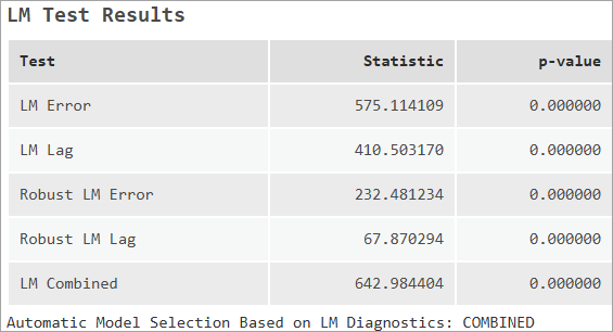
First, the LM test for the spatial lag (LM Lag) and for the spatial error (LM Error) models are performed. If neither tests are statistically significant (p-value greater than 0.05), a spatial model is not necessary, and an OLS model is selected. If only one of the tests is significant, the corresponding model is selected.
If both the LM Lag and LM Error tests are significant, their robust counterparts are performed. These are the Robust LM Lag and the Robust LM Error tests, which are slightly more stringent forms of the test. If only one of the tests is significant, the corresponding model is selected.
If both of robust tests are significant, an LM test for the SAC model is performed. In the case that all three tests are significant, the model with the largest test statistic is chosen.
In the rare case that both the LM Lag and LM Error tests are significant but neither of the robust tests are significant, the SAC model is chosen.
It is important to note that the LM tests are a data-driven approach to choosing a model. They do not guarantee a good model or fit. Review the diagnostics and consider the theoretical assumptions of the model.
Tool outputs
The primary output of the tool is a number of tables in the geoprocessing messages as well as an output feature class and a chart visualizing the residuals of the model.
Output features
The output feature class of the tool will contain fields of the dependent variable, explanatory variables, the predicted value of the dependent variable, residual and standardized residual, the spatial lag of the residual, and the number of neighbors of each feature.

When the layer is added to a map, the features will be shaded by their standardized residuals. Visualizing the standardized residuals can assist in identifying any patterns of clustering in the error term.

The residuals are symbolized from a deep purple to a dark green. Locations symbolized with green have a positive residual meaning that the model overestimated the value. Similarly, locations with a purple color have a negative standardized residual. Negative residuals indicate a location that is underestimated.
Moran's Scatter Plot of Residuals
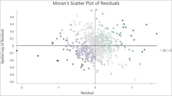
The output layer contains a scatter plot chart displaying the residuals plotted against their spatial lag. The x-axis displays the standardized residual, and the y-axis displays the spatial lag of the standardized residual. This type of chart is referred to as a Moran's scatter plot.

The chart can be split into four quadrants around 0 on the x and y axes. Values in the top-right and lower-left quadrants exhibit positive spatial autocorrelation. These are locations that have similar values as their neighbors: positive and negative values respectively. The top-left and bottom-right quadrants are locations that exhibit negative spatial autocorrelation. These are locations that have high values surrounded by low-values (and vice versa).
When the residuals are evenly distributed across the four quadrants, it indicates that there is no discernible spatial autocorrelation. This type of pattern is expected when the regression model performed well and the majority of spatial autocorrelation has been accounted for.
Geoprocessing messages
The tool provides a number of tables in the geoprocessing messages that provide insight into the how each model is estimated:
- Neighborhood and Spatial Weights Summary
- LM Test Results
- Summary of Model Results
- Model Diagnostics
In some cases, the following message tables will also be displayed:
- Coefficient Effects Summary
- Coincident Point Report
Each table is described in the following sections.
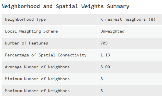
Neighborhood and Spatial Weights Summary
The SEM, SLM, and SAC models require a spatial weights matrix, which can heavily influence the model results. The Neighborhood and Spatial Weights Summary table provides insight into the spatial weights matrix used to fit the model. It reports the neighborhood type, weighting scheme, spatial connectivity, average neighborhood size, minimum neighborhood size, and maximum neighborhood size.

It is important to note that the tool will not estimate a model if the spatial weights matrix is too connected. The percentage of spatial connectivity is approximately the average number of neighbors for each feature, as a percent of the total number of features. For example, with 500 features and spatial connectivity equal to 0.1, each feature will have approximately 50 neighbors on average. If the spatial weights matrix has a connectivity of 30 percent or greater, the model results will become biased (Smith, 2009). In this case, the tool will return an error.
LM Test Results
The LM Test Results table reports the Lagrange Multiplier diagnostics for each of the tests. The table also displays the model type that would be selected based on the flow chart in the Choosing the appropriate model section above.

Coincident Point Report
Coincident points (points with the same coordinates) can cause various issues in spatial regression, such as creating weights equal to zero for all neighbors. If coincident points are present in your input features, a Coincident Point Report will be displayed that reports the total features, the number of unique locations, as well as the minimum, maximum, and average number of coincident points for all features. Additionally, warnings and errors caused by the coincident points may be displayed.

Model Diagnostics
The Model Diagnostics table displays important diagnostics, such as the dependent variable, the number of features, degrees of freedom, as well as which model was used.

If an OLS model is estimated, the adjusted R-squared is displayed in the table. However, for all spatial models, a pseudo R-squared is displayed instead. For the SLM and the SAC models, a spatial pseudo R-squared is also displayed. These are discussed below.
Additionally, the Jarque-Bera statistic is also reported. If the statistic is significant, it indicates that the model’s residuals are not normally distributed. While the models are estimated using methods robust to non-normality, the test may indicate a model misspecification or the presence of outliers.
Interpret spatial lag model results
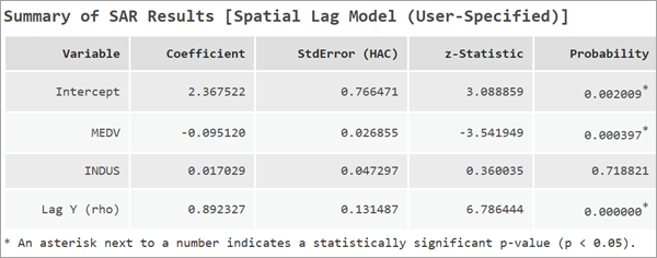
The spatial lag model reports an additional coefficient called Lag Y (rho). This is the spatial lag of the dependent variable. The coefficient of this variable measures the strength and direction of spatial dependence of the dependent variable. The value of rho must be between -1 and 1. Larger values of Lag Y suggest a strong spatial feedback process.

It is important to note that a change in an explanatory variable in one location can affect the value of the dependent variable in another location, called spatial spillover. In the presence of spatial spillover, the regression coefficients must be interpreted along with the spatial spillover effect.
Impacts and coefficient effects
In addition to regression coefficients, a measure called impacts are reported. Impacts help measure the effect of spatial spillovers for each explanatory variable. They are broken down into direct, indirect, and total impacts. There are different approaches to calculating impacts, and this tool reports simple impacts. The direct, indirect, and total impacts are displayed in the Coefficient Effects Summary message table.

The direct impact measures how much a one unit change in an explanatory variable affects the value of the dependent variable at the location itself. In the case of simple impacts, this is the same value as the beta coefficient.

Whereas the indirect impact measures how much a one unit change in a variable affects the dependent variable in its neighboring locations. Note, however, that the value of impacts is strongly influenced by the spatial weights matrix.
Standard errors
By default, the spatial lag model reports robust standard errors. However, after fitting a spatial lag model, a large amount of autocorrelation in the residuals may remain. The Anselin-Kelejian (AK) test is a diagnostic test that is used to determine if a significant amount of spatial dependence remains in the model residuals.

If the AK test is significant (p-value less than 0.05), a different measure of standard error, called heteroskedastic and autocorrelation robust (HAC) standard errors, are reported. HAC standard errors are a nonparametric variant of standard errors that are useful in the presence of spatial autocorrelation.

HAC standard errors take into account the spatial distribution of the data by using a separate spatial weights matrix. The spatial weights matrix is created using k nearest neighbors to identify each feature’s neighborhood with the focal feature included in the neighborhood. The weights of each neighborhood are modeled using a triangular kernel.
Pseudo R-squared and spatial pseudo R-squared
Because the spatial lag model includes the spatial lag of the dependent variable as an explanatory variable, traditional linear regression prediction methods cannot be used. Predicting the dependent variable using its spatial lag leads to overconfident estimates. To overcome this, another measure called the spatial pseudo R-squared is calculated.
The spatial pseudo R-squared is calculated without the spatial lag of the dependent variable. Instead, it uses the spatial weights matrix and the estimate of λ to create a predicted values of Wy-hat that is used in place of Wy in the prediction.
The predicted values are then used to calculate a traditional pseudo R-squared value. It is recommended that you report the spatial pseudo R-squared value over the pseudo R-squared value.
It is important to note that the spatial pseudo R-squared is a different measure than the adjusted R-squared that is reported by OLS results. As such, it is inappropriate to compare the two.
Interpret spatial error model results
In the spatial error model, the regression coefficients can be interpreted similarly to those in standard linear regression. Each coefficient represents the change in the dependent variable for a one-unit change in the independent variable. However, the SEM also includes an additional component, Lag Residual (lambda), which plays a crucial role in understanding spatial dependence within the model. The coefficient of Lag Residual (lambda) will always be between -0.99 and 0.99.

A positive value of lambda suggests that the residuals exhibit spatial clustering, and a negative value of lambda indicates that the residuals exhibit spatial dispersion. Larger absolute values (positive or negative) of lambda also suggest that there are spatial processes that are unaccounted for by the explanatory variables. Including additional relevant explanatory variables may reduce the coefficient to more moderate levels.
Interpret spatial autoregressive combined model results
When the SAC model is selected, all sections applicable to the SLM and the SEM models are displayed in the messages.

References
The following resources were used to implement the tool:
- Anselin, L., and Sergio J. Rey. 2014. "Modern spatial econometrics in practice: A guide to GeoDa, GeoDaSpace and PySAL." ISBN 9780986342103.
Bivand, Roger and Gianfranco Piras. 2015. "Comparing implementations of estimation methods for spatial econometrics." Journal of Statistical Software. 63: 1-36. https://doi.org/10.18637/jss.v063.i18.
Kelejian, Harry H., and Ingmar R. Prucha. 2007. "HAC estimation in a spatial framework." Journal of Econometrics. 140, no. 1: 131-154. https://doi.org/10.1016/j.jeconom.2006.09.005.
Smith, Tony E. 2009. "Estimation bias in spatial models with strongly connected weight matrices." Geographical Analysis. 41, no. 3: 307-332. https://doi.org/10.1111/j.1538-4632.2009.00758.x.