Creating a space-time cube allows you to visualize and analyze spatiotemporal data, in the form of time-series analysis, integrated spatial and temporal pattern analysis, and 2D and 3D visualization techniques. There are three primary tools that create a space-time cube for analysis: Create Space Time Cube By Aggregating Points, Create Space time Cube From Defined Locations, and Create Space Time Cube From Multidimensional Raster Layer. The first two tools structure time-stamped features into a netCDF data cube by generating space-time bins with either aggregated incident points or defined features with associated spatiotemporal attributes. The third tool converts a time-enabled multidimensional raster layer to a space-time cube and does not perform spatial or temporal aggregation.
If you have time-stamped point features that you want to aggregate spatially to understand spatiotemporal patterns at locations throughout a study area, use the Create Space Time Cube By Aggregating Points tool. This will result in either a grid cube (fishnet or hexagon) or a cube structured by the defined locations you provide as aggregation polygons. In each bin of the cube, the points are counted, Summary Field statistics are calculated, and the trend for bin values across time at each location is measured using the Mann-Kendall statistic. When you aggregate using a fishnet or hexagon grid, a grid cube is created. When you aggregate using a set of defined locations as aggregation polygons, a defined locations cube is created. Creating a space-time cube by aggregating points is most common when the point data represents incidents—such as crimes or customer sales, for example—and you want to aggregate those incidents into either a grid or a set of polygons representing police beats or sales territories, respectively.
If you have feature locations that do not change over time and attributes or measurements that have been collected over time, such as panel data or station data, use the Create Space Time Cube From Defined Locations tool. This will result in a cube that is structured using those defined locations, with either one set of attributes per time period (if no temporal aggregation is chosen) or summary statistics at each time period for the attributes chosen (if temporal aggregation is chosen). In each bin of the defined locations cube, the count of observations for that bin at that time period and any Variables or Summary Field statistics are calculated, and the trend for bin values across time at each location is measured using the Mann-Kendall statistic.
If you have a multidimensional raster and want to perform space-time analysis using the tools in the Space Time Pattern Mining toolbox, use the Create Space Time Cube From Multidimensional Raster Layer tool to convert the multidimensional raster to a space-time cube. If the raster cells are squares (their cell sizes in x and y are equal), the output space-time cube will be a grid cube. If the raster cells are rectangular, the output space-time cube will be a defined locations cube. The output space-time cube will have the same spatial and temporal resolution as the multidimensional raster in which each raster cell of each dimension is converted to a single space-time bin. Trends in the values across time will be analyzed using the Mann-Kendall statistic. Most information in this topic does not apply to this tool because the structure of the space-time cube is defined by the structure of the multidimensional raster and cannot be changed.
The Subset Space Time Cube tool and all of the tools in the Time Series Forecasting toolset can also create space-time cubes. The Subset Space Time Cube tool creates a space-time cube that follows the structure of the input cube except where the spatial or temporal extent was subsetted by the tool. The time series forecasting tools create a space-time cube that follows the spatial structure of the input cube but extends the temporal extent to include the forecast time steps. Most information in this topic does not apply to these tools because the structure of the space-time cube is defined by the structure of the input space-time cube and cannot be changed.
Set the structure of the cube
In most cases, you will know how to define the cube bin dimensions; it is recommended that you consider what the appropriate dimensions should be for the particular questions you are trying to answer. If you are reviewing crime events, for example, you may decide to aggregate points into 400-meter or 0.25-mile bins because that is a city block size. If you have data covering an entire year, you may decide to review trends in terms of monthly or weekly event aggregation.
Grid cube
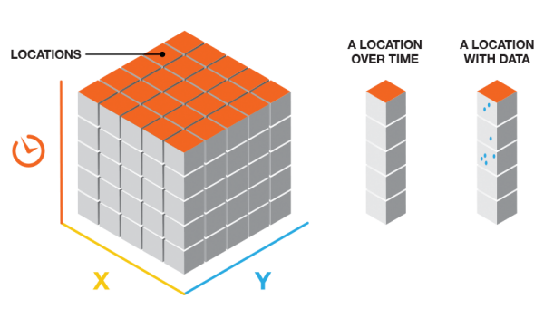
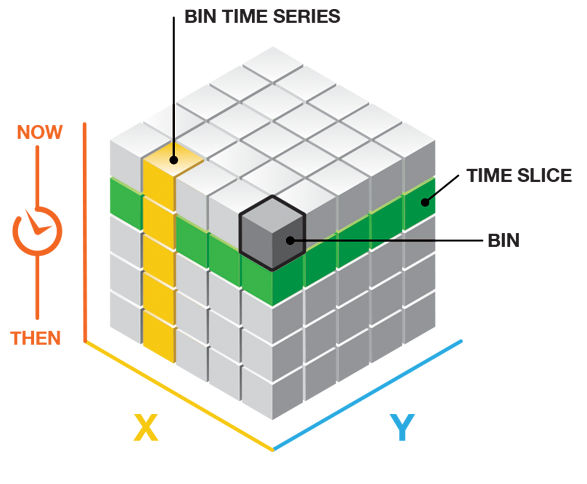
The grid cube structure has rows, columns, and time steps. If you multiply the number of rows by the number of columns by the number of time steps, you will obtain the total number of bins in the cube. The rows and columns determine the spatial extent of the cube, and the time steps determine the temporal extent.
Defined locations cube
The defined locations cube structure has features and time steps. If you multiply the number of features by the number of time steps, you will obtain the total number of bins in the cube. The features determine the spatial extent of the cube, and the time steps determine the temporal extent.
Multidimensional raster layer cube
The multidimensional raster layer cube structure has the same number of features and time dimensions as the number of cells and dimensions of the multidimensional raster layer.
Spatial structure
Spatial defaults for the grid cube
When you do not have strong justification for a particular grid size for a grid cube, you can leave the Distance Interval parameter blank, and the tool will calculate default values.
The default bin distance is calculated by first determining the distance of the longest side of the Input Features extent (maximum extent). The bin distance set is then the larger of either the maximum extent divided by 100 or an algorithm based on the spatial distribution of the input features.
Spatial structure of the defined locations cube
The spatial structure of the defined locations cube is the provided locations.
Spatial structure of the multidimensional raster layer cube
The spatial structure of the multidimensional raster layer cube is defined by the spatial extent and resolution of the multidimensional raster layer.
Temporal structure
Temporal defaults for the grid cube
When you do not have strong justification for a particular time-step interval, you can leave the Time Step Interval parameter blank, and the tool will calculate default values. The default time-step interval is based on two different algorithms used to determine the optimal number and width of time-step intervals. The minimum numeric result from these algorithms, greater than 10, is used for the default number of time-step intervals. If both numeric results are less than 10, 10 becomes the default number of time-step intervals.
Temporal structure of the defined locations cube
You must specify the temporal structure of the defined locations cube. If your data is collected every 5 years, for example, specify that in the Time Step Interval parameter.
You can also aggregate temporally in a defined locations cube. If you have stations that are recording moisture readings every 5 minutes, for example, you can use Temporal Aggregation to combine those readings into hourly averages.
If temporal aggregation is chosen, you can assess the aggregation by mapping the number of features aggregated into each bin. For instance, if you have data collected every 5 minutes and you are aggregating into hourly averages, you would expect to see 12 features aggregated into each hour in each bin. If you use the Visualize Space Time Cube in 3D tool to map the Temporal Aggregation Count Cube Variable and see that you have several bins with values less than 12, that indicates that some of the moisture readings were not present. This is not necessarily a problem but valuable to understand if one of the sensors has a problem or if a location has too much missing data over time to be included in the analysis.
Temporal structure of the multidimensional raster layer cube
The temporal structure of the multidimensional raster layer cube is defined by the time dimensions of the multidimensional raster layer.
Time-step alignment
When creating a defined locations cube with no temporal aggregation, the only consideration is choosing Time Step Interval, Time Step Alignment, and Reference Time values that ensure that only a single record falls within each bin. The issue of temporal bias is not present.
If you are not aggregating and want to create monthly time-step intervals and the data falls between the first of the month and the sixth of the month due to collection procedures, the best practice is to use the Reference Time option for Time Step Alignment and choose a date that ensures that one month forward and backward will include each data point. For example, if you have data on 1/1, 2/3, 3/2, 4/1, and 5/3, choosing a reference time on the first of any month in the dataset will ensure that all data is appropriately included in the resulting cube.
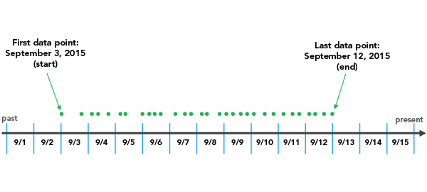
When you are aggregating data into a space-time cube, the Time Step Alignment parameter is important because it determines where the aggregation will begin and end. See the following example:
End time
If an End time value is set for Time Step Alignment with a Time Step Interval value of three days, for example, the binning will initiate with the last data point and go back in three-day increments until all data points fall within a time step.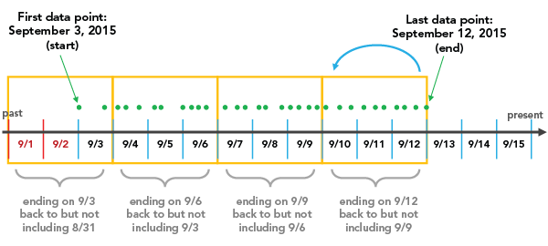
Depending on the Time Step Interval value you choose, you can create a time step at the beginning of the space-time cube that does not have data across the entire time span. In the example above, 9/1 and 9/2 are included in the first time step even though no data exists until 9/3. These empty days are part of the time step but have no data associated with them. This can bias the results because it will appear that the temporally biased time step has significantly fewer points than other time steps, which is an artificial result of the aggregation scheme. The report indicates whether there is temporal bias in the first or last time step. In this case, two out of the three days in the first time step have no data, so the temporal bias is 66 percent.
End time is the default option for Time Step Alignment because many analyses are focused on what has occurred most recently, so putting this bias toward the beginning of the cube is preferable. Another solution, which completely removes the temporal bias, is to provide data that is divided evenly by the Time Step Interval value so that no time periods are biased. You can do this by creating a selection set of the data that excludes the part of the point dataset that falls outside of what you want to be the first time period. In this example, selecting all data except that of 9/3 and before solves the problem. The report shows the time span of the first and last time steps, and that information can be used to determine the cutoff date.
If, in the process of moving back in time, the final bin lands exactly on the first data point as its start, that final data point is not included in that bin. This is because, with an End time value for Time Step Alignment, each bin includes the last date in a given bin, yet goes back to but does not include the first date in that bin. In this case, an additional bin must be added to ensure that the first data point is included.
Start time
If a Start time value is set for Time Step Alignment with a Time Step Interval value of thee days, for example, binning will start at the first data point and continue in three-day increments until the last data point falls within the final time step.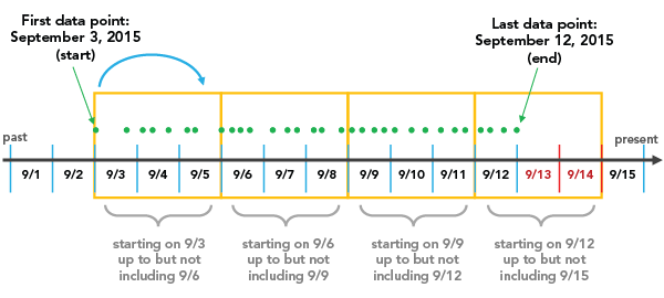
There are a few things to note. One is that with a Start time value for Time Step Alignment based on the Time Step Interval value that you choose, you can create a time step at the end of the space-time cube that does not include data across the entire time span. In the example above, 9/13 and 9/14 are included in the last time step even though no data exists after 9/12. These empty days are part of the time step but have no data associated with them. This can bias the results because it will appear that the temporally biased time step has significantly fewer points than other time steps, which is an artificial result of the aggregation scheme. The report indicates whether there is temporal bias in the first or last time step. In this case, two out of the three days in the last time step have no data, so the temporal bias is 66 percent. This is problematic when choosing a Start time value for Time Step Alignment because analyses that are focused on the most recent data can be impacted. The solution is to provide data that is divided evenly by the Time Step Interval value so that no time periods are biased. You can do this by creating a selection set of the data that excludes the part of the point dataset that falls outside of what you want to be the last time period. In this example, selecting all data except that of 9/12 and after solves the problem. You can also remove two days from the beginning of the dataset, which also leads to the data falling evenly within the time steps. The report shows the time span of the first and last time steps, and that information can be used to determine the cutoff date.
If, in the process of moving forward in time, the final time step lands exactly on the last data point as its end, that final data point is not included in that bin. This is because, with a Start time value for Time Step Alignment, each bin includes the first date in a given bin, yet goes forward to but does not include the last date in that bin. In this case, an additional bin must be added to ensure that the last data point is included.
Reference time
A Reference time value for Time Step Alignment allows you to ensure that a specific date marks the beginning or end of one of the time steps in the cube.
When you choose a Reference time value that falls
after the extent of the dataset—at the last data point or in the
middle of the dataset—it is treated as the last data point of
a time step, and all other bins on either side are created using
Time Step Alignment until all of the data is covered
as illustrated below.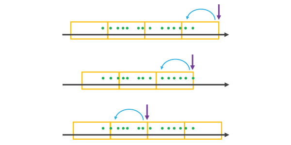
When you choose a Reference time value that falls before the extent of the dataset or at the first data point, it is treated as the first data point of a time step, and all other time steps on either side are created using a Start time value for
Time Step Alignment until all of the data is covered as illustrated below.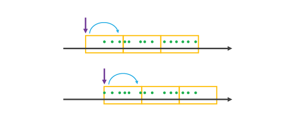
Choosing a Reference time value before or after the temporal extent of the data can create empty or partially empty bins, which can bias the analysis.
Template cubes for grid cubes
Note:
A template cube cannot be used with defined locations cubes. They are only applicable to grid cubes.
Choosing a Template Cube value has implications for
the Time Step Alignment parameter. When you
choose a Template Cube value that falls before or after the time span of
Input Features, time steps are added until all of the data
is covered by a time step using the Time Step Alignment value of the
template cube. The resulting space-time cube will have empty cubes
wherever the Template Cube value did not overlap the Input Features value in
time. This can bias the results of the analysis. If the template cube
overlaps the input features, the resulting space-time cube will
cover the temporal extent of the template cube and extend until all
input features are covered using the time-step alignment of the
template cube. The illustration below shows template cubes in blue
and the resulting space-time cubes in orange.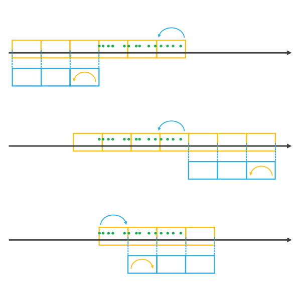
When creating a space-time cube using the Template Cube option, the temporal extent of the template cube will be extended until all data is covered. This allows you to use last year's cube to create a cube that includes both last year's data and this year's data. The spatial extent of the template cube is treated differently. Any data falling outside of the spatial extent of the template cube will be excluded from the analysis. The template cube and the resulting space-time cube will have identical spatial extents. The only changes that can occur are within the spatial extent where locations that previously had no data can become locations with data if new features have appeared that were not present when the template cube was created.
Attributes
The attributes of a space-time cube depend on how the cube is created.
Aggregate points
When creating a cube by aggregating points, whether a grid cube or a defined locations cube, a COUNT field is calculated specifying the number of points in each bin. In addition to the COUNT field, you can summarize attributes in each bin. Multiple statistic and field combinations can be specified. Null values are excluded from all statistical calculations. When choosing Summary Fields, each location must have a value for each attribute at every time step. You can choose how the tool fills empty bins (bins that have no points and no attribute values) using the Fill Empty Bins with parameter. Multiple options are available, and you can choose a different fill type for each field being summarized. Bins that cannot be filled based on the estimation criteria will result in the entire location being excluded from the analysis. A minimum of 4 neighbors are required to fill empty bins using the average value of spatial neighbors, and a minimum of 13 neighbors are required to fill empty bins using the average value of space time neighbors.
Defined locations
When creating a cube from defined locations with no temporal aggregation, you choose the variables from the data that you want to include in the cube, and a Fill Empty Bins with option that is most appropriate if there are null values or missing features at particular time periods in the dataset and you do not want the locations to be excluded.
When creating a cube from defined locations with temporal aggregation, choose the Summary Fields values that you want to include in the resulting cube and the Statistic type that will be used to summarize them. Because each location must have a value at every time step, in addition to choosing a Statistic type, you must also choose how to complete the time series using the Fill Empty Bins with parameter. Multiple options are available, and you can choose a different fill type for each field being summarized.
Statistic types (defined locations and aggregating points cubes)
The available statistic types are as follows:
- SUM—Adds the total value for the specified field within each bin
- MEAN—Calculates the average for the specified field within each bin
- MIN—Finds the smallest value for all records of the specified field within each bin
- MAX—Finds the largest value for all records of the specified field within each bin
- STD—Finds the standard deviation on values in the specified field within each bin
- MEDIAN—Finds the sorted middle value of all records of the specified field within each bin
Caution:
Null values present in any of the summary fields will result in those features being excluded from analysis. If having the count of points in each bin is part of your analysis strategy, consider creating separate cubes, one for the count (without summary fields) and one for summary fields. If the set of null values is different for each summary field, consider creating a separate cube for each summary field.
Fill Empty Bins with (for all cubes)
The available fill types are as follows:
- Zeros—Fills empty bins with zeros
- Spatial neighbors—Fills empty bins with the average value of spatial neighbors
- Space-time neighbors—Fills empty bins with the average value of space-time neighbors
- Temporal trend—Fills empty bins using an interpolated univariate spline algorithm
When using the Create Space Time Cube From Defined Locations tool, there is an additional Drop locations fill type that excludes locations with missing data for any of the variables from the output space-time cube.
Interpret results
Messages
In addition to the netCDF file, messages summarizing the space-time cube dimensions and contents appear at the bottom of the Geoprocessing pane during tool operation. To access the messages, hover over the progress bar and click the pop-out button  , or expand the messages section in the Geoprocessing pane. You can also access the messages for a previously run tool through the geoprocessing history.
For grid cubes, only locations with data for at least one time-step interval are included in the analysis, but they are analyzed across all time steps. When computing point counts in a grid cube, zero counts are assumed for any bin in which there are no points but the associated location has had at least one point for at least one time-step interval. Information about the percentage of zeros associated with locations that have data for at least one time-step interval is reported in the messages as sparseness.
For defined locations, any location that has a complete time series is included in the defined locations cube even if that time series is entirely composed of zeros. This is important to consider if you aggregated points into defined locations.
At the end of the output message, there is information about the overall data trend. This trend is based on an aspatial time-series analysis. The question it answers is, overall, are the events represented by the input increasing or decreasing over time? To obtain the answer, all locations in each time-step interval are analyzed together as a time series using the Mann-Kendall statistic.
Trend analysis
The Mann-Kendall trend test is performed on every location with data as an independent bin time-series test. The Mann-Kendall statistic is a rank correlation analysis for the bin count or value and their time sequence. The bin value for the first time period is compared to the bin value for the second. If the first is smaller than the second, the result is +1. If the first is larger than the second, the result is -1. If the two values are tied, the result is zero. The result for each pair of time periods compared are summed. The expected sum is zero, indicating no trend in the values over time. Based on the variance for the values in the bin time series, the number of ties, and the number of time periods, the observed sum is compared to the expected sum (zero) to determine whether the difference is statistically significant. The trend for each bin time series is recorded as a z-score and a p-value. A small p-value indicates that the trend is statistically significant. The sign associated with the z-score determines if the trend is an increase in bin values (positive z-score) or a decrease in bin values (negative z-score). Strategies for visualizing the trend results are provided in Visualize the space-time cube.
Visualization
You can visualize the space-time cube data in either 2D or 3D by using the Make Space Time Cube Layer to create a space-time cube layer. The layer allows you to quickly visualize and explore 3D Space Time Pattern Mining analysis results. The tool takes a space-time cube as input and creates layers that can be visualized in a number of ways. There are many display options available, all with preset symbology and range and time sliders that make the exploration of the space-time cube and analysis results intuitive. Three-dimensional visualizations of the space-time cube can also be displayed as web scenes and shared in stories using ArcGIS StoryMaps.
Additional resources
The creation, visualization, and analysis of the space-time cube utilizes netCDF software developed by UCAR/Unidata.
Learn more about Unidata and the Network Common Data Form (NetCDF) project
For information about histogram bin-width optimization, see the following:
- Shimazaki H. and S. Shinomoto, "A method for selecting the bin size of a time histogram," Neural Computation Vol. 19(6), (2007): 1503–1527.
- Terrell, G. and D. Scott, "Oversmoothed Nonparametric Density Estimates," Journal of the American Statistical Association Vol. 80(389), (1985): 209-214.
- Online Statistics Education: A Multimedia Course of Study (http://onlinestatbook.com/). Project leader: David M. Lane, Rice University (chapter 2, "Graphing Distributions, Histograms").
For information about the Mann-Kendall trend test, see the following:
- Hamed, K. H., "Exact distribution of the Mann-Kendall trend test statistic for persistent data," Journal of Hydrology (2009): 86–94.
- Kendall, M. G. and J. D. Gibbons, Rank correlation methods, fifth ed., (1990) Griffin, London.
- Mann, H. B., "Nonparametric tests against trend," Econometrica Vol. 13, (1945): 245–259.