The Time Series Clustering tool identifies the locations in a space-time cube that are most similar and partitions them into distinct clusters in which members of each cluster have similar time series characteristics. Time series can be clustered so they have similar values across time, stay in proportion across time, or display similar smooth periodic patterns across time. This tool takes a space-time NetCDF cube as input that can be created using the Create Space Time Cube By Aggregating Points, Create Space Time Cube From Defined Locations, or Create Space Time Cube From Multidimensional Raster Layer tools. The tool generates a 2D feature class displaying each location in the cube symbolized by its cluster membership, as well as informative messages. Optionally, the Output Table for Charts and Enable Time Series Pop-ups parameters can be used to create charts that show representative time series for each cluster and the time series for each location of the space-time cube.
Potential applications
- An analyst has created a space-time cube representing several years of 911 calls and can use the Time Series Clustering tool with the Value option of Characteristics of Interest to determine which neighborhoods have similar call volumes.
- A large retailer might use this tool with Profile (Correlation) as the Characteristics of Interest value to find stores that have similar purchasing patterns. For example, this tool helps users distinguish the stores whose sales increase during the Christmas shopping season and decrease after Christmas from the stores whose sales don't have this pattern. The stores with different sales patterns are worth further investigation. This information can be also used to help the retailer predict demand and ensure that stores have sufficient inventory.
- A meteorologist might use this tool with Profile (Fourier) as the Characteristics of Interest value to cluster places based on how close their temperatures fluctuate together over time and how similar the extent of their fluctuation.
- Demographers might use this tool to evaluate which countries have similar patterns of population growth, both in terms of value and profile of time series.
Tool outputs
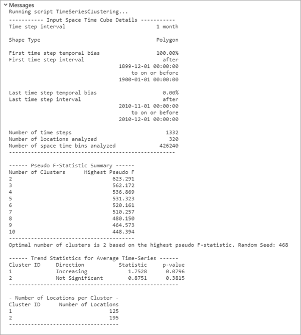
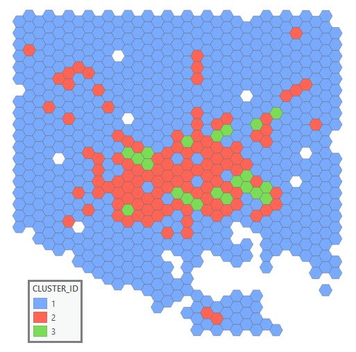
A number of outputs are created by this tool. A 2D feature class showing each location in the Input Space Time Cube, symbolized by its cluster membership allows you to explore any spatial patterns. Even though the clustering algorithms used in this tool do not take any spatial relationships into account when performing the clustering, there may still be spatial patterns present. In addition, messages summarizing the analysis results and Mann-Kendall trend statistics for each cluster are written at the bottom of the Geoprocessing pane during tool execution.
You can access the messages by hovering over the progress bar, clicking the pop-out button  , or expanding the messages section in the Geoprocessing pane. You can also access the messages for a previously run tool using geoprocessing history.

The default output of the Time Series Clustering tool is a new output features class containing the CLUSTER_ID field, which indicates to which cluster each location belongs. This output feature class is added to the Contents pane with a unique color rendering scheme applied to the CLUSTER_ID field. The CENTER_REP field indicates which locations in the space-time cube are most representative of each cluster (called the medoids of the clusters). This field will contain a value of 1 for the medoid of each cluster, and all other locations will contain a value of 0.

Time Series Clustering chart outputs
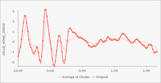
Charts are produced when you create an Output Table for Charts. The Average Time Series per Cluster chart displays the average of Analysis Variable at each time step for each cluster, and the Time Series Cluster Medoids chart displays the medoid time series of each cluster. Together, these charts allow you to visualize both the overall average and the representative time series broken down by cluster. This is analogous to summarizing the categories of a univariate dataset using the mean and the median.

You can also use the Enable Time Series Pop-ups parameter to create time series charts in the pop-ups of each output feature that show the time series of the feature and the average time series of all features in the same cluster. This allows you to see how the time series of the feature compares to other features in the same cluster and how well it is represented by the cluster.

Similarity between time series
The goal of clustering is to partition the locations of the space-time cube into groups in which the time series of locations within each group are more similar to each other than they are to the time series of locations outside the group. However, time series are composed of many numbers or values across time, so it is not completely clear what it means for two time series to be similar. For individual numbers, a useful measure of similarity is the absolute difference in their value: the difference between 10 and 13 is 3. You can say that 10 is more similar to 13 than it is to 17 because the absolute difference in their values is smaller. For time series, however, similarity is less obvious. For example, is the time series (5, 8, 11, 7, 6) more similar to (4, 9, 13, 4, 9) than it is to (5, 11, 6, 7, 6)? To answer a question like this, you must be able to measure how similar or different two time series are. There are several ways to measure similarity, and each depends on which characteristics of the time series you consider important. The characteristic you choose will be the characteristic that will be most similar between locations in the same output clusters.
The Characteristic of Interest parameter is used to specify the characteristic of the time series you want to be similar within each cluster. Clustering can be based on one of three characteristics.
Value characteristic
The Value option of the Characteristic of Interest parameter is the simplest option, and it is used to cluster time series that have similar values over time.
This option measures the similarity of the time series using the Euclidean distance between the values in the time series (not to be confused with the distance in space between the locations of the two time series). For example, the difference between the time series (1, 5, 2, 3) and (3, 1, 3, 5) is 5. This value is calculated by taking the square root of the sum of squared differences in values across time:
SquareRoot[ (1-3)2 + (5-1)2 + (2-3)2 + (3-5)2 ] = 5Profile (Correlation) characteristic
The Profile (Correlation) option of the Characteristic of Interest parameter is used to cluster time series that tend to stay in proportion to each other and increase and decrease in value at the same time. For example, you can use this option to cluster store branches based on their growth rates. Even if their actual values are very different, locations will cluster together if they follow similar growth patterns.
This option measures the similarity in time series based on their statistical correlation across time. For example, the time series (1, 2, 3, 4, 5) has very different values than the time series (10, 20, 30, 40, 50), but they are perfectly correlated, and their difference is 0. This difference between two time series is calculated by subtracting the correlation from 1. This means that time series that are perfectly positively correlated (correlation = 1) have a difference of 0, time series that are uncorrelated (correlation = 0) have a difference of 1, and time series that are perfectly negatively correlated (correlation = -1) have a difference of 2. All other degrees of correlation result in values between 0 and 2, with larger positive correlations indicating higher similarity.
Profile (Fourier) characteristic
The Profile (Fourier) option of the Characteristic of Interest parameter is the most complicated option, and it is used to cluster time series that have similar smooth, periodic patterns in their values across time. These periods are sometimes called cycles or seasons, and they represent durations of a single pattern that then repeats in a new period. For example, temperature follows a consistent yearly period with higher temperatures in the summer and lower temperatures in the winter, and this option could be used to find areas that have most similar yearly temperature patterns.
Optionally, you can ignore certain characteristics of these patterns with the Time Series Characteristics to Ignore parameter. You can ignore the starting times of these periods so that only the shapes and durations of the periods are compared, and you can ignore the magnitude of the values within the periods so that you only compare the starting times and durations of the periods. If you ignore both characteristics, two time series will be considered similar if the durations of their periods are approximately the same, even if the periods start at different times and have different values within the periods.
The Profile (Fourier) option measures similarity between time series using concepts from functional data analysis. Each time series is decomposed into a sequence of basis functions that represent the most dominant signals in the time series. The Fourier family of basis functions use sine and cosine functions that oscillate up and down at a constant interval to represent the time series. Each basis function has an associated weight that measures the prevalence of that particular signal in the time series. For example, temperature displays two dominant basis functions, one that oscillates up and down corresponding to days and nights, and the other oscillates according to seasons of the year. Basis functions corresponding to other intervals would receive lower weights because they are not prevalent in the time series of temperatures. For example, a basis function that oscillates up and down every 90 minutes would have a small associated weight because temperature does not naturally change at that interval. For this option to be most effective, the time series should span the duration of at least one period. For example, the dominant yearly period for temperature would likely not be captured if the data were only measured within a few months. For N locations in the space-time cube, the tool will use N-2 basis functions if N is even and N-1 basis functions if N is odd.
The difference between two time series is calculated by summing the squared differences between the weights of the associated basis functions of each time series. This means that two time series that have similar dominant oscillating signals will be considered similar.
Clustering time series by similarity
While some options are more complicated than others, all options of the Characteristic of Interest parameter calculate a single number that measures the difference between two time series. Using this definition of similarity between time series, the locations of the space-time cube are clustered using one of several clustering algorithms.
See the Additional references section below for comprehensive details of the clustering algorithms.
Clustering Profile (Correlation)
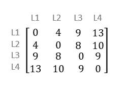
If the Profile (Correlation) option of the Characteristic of Interest parameter is chosen, the difference between every pair of locations in the space-time cube is calculated summarized as a dissimilarity matrix. An example of a dissimilarity matrix is shown below for the time series of four locations, labeled L1, L2, L3, and L4. A time series is always considered exactly the same as itself, and this is indicated by the zeros along the diagonal of the matrix. The matrix is also symmetric because the difference between two time series does not depend on their ordering: the difference between A and B is the same as the difference between B and A. For the dissimilarity matrix below, locations L1 and L2 are most similar (indicated by the value 4), and time series L1 and L4 are most different (indicated by the value 13).

This matrix is then clustered using the k-medoids algorithm, also called the Partitioning Around Medoids (PAM) algorithm. This algorithm finds clusters within the matrix in which members of the clusters are more similar than members of other clusters. This algorithm is random in nature, and it works by choosing random locations to serve as representatives of each cluster. These representatives are called medoids, and they are analogous to the median of a univariate dataset. Initial clusters are created by assigning every other location to the cluster whose medoid is most similar. The algorithm then swaps medoids within each cluster and reevaluates the similarity within the new clusters. If the new clusters are more similar than the initial clusters, the medoids are swapped, and the process repeats until there are no swaps that will increase the similarity of the clusters. While the final clusters will almost always have high similarity, the clusters can be different depending on the random locations that were chosen as initial medoids. Running the tool several times can produce modestly different clustering, so you are encouraged to run the tool several times to see different possible clustering results.
If there are more than 10,000 locations in your space-time cube, the tool will use a variant of k-medoids called Clustering LARge Applications (CLARA). CLARA works by taking a random sample of the time series and performing the k-medoids algorithm. All locations that were not chosen in the random sample are then assigned to the cluster whose medoid is most similar to the time series of the unsampled location. The size of the random sample is the larger of two values: the square root of the number of locations (rounded down), or 40 + 2k, where k is the number of clusters.
Clustering Value and Profile (Fourier)
If the Value or Profile (Fourier) options of the Characteristic of Interest parameter are chosen, the locations of the space-time cube are clustered using the k-means algorithm. This algorithm is conceptually similar to k-medoids, but it can be performed without calculating the difference between every pair of locations. Instead, it will start by randomly selecting locations as representatives of each cluster. Initial clusters are then generated by assigning all remaining locations to the cluster whose representative is most similar to the location. A new representative for each cluster is then calculated by averaging the time series within each cluster. For Value, this new representative is the average of each time step of each time series in the cluster. For Profile (Fourier), this new representative is the average of the weights of each basis function. Unlike k-medoids, these new representatives will generally not correspond to any individual location in the space-time cube. Each time series is again assigned to the cluster whose representative is most similar, and new average representatives are calculated. This process repeats until the algorithm converges, meaning that the clusters do not change after the repetition. At this point, continuing the process would result in the same clusters over and over. These are the clusters that are returned by the tool.
As with the k-medoids algorithm above, the k-means algorithm can provide different clustering results depending on the initial random cluster representatives. You are encouraged to run the tool several times to see different possible clustering results.
Optimal number of clusters
When you leave the Number of Clusters parameter empty, the tool will evaluate the optimal number of clusters, and the value will be reported in the messages window. Determining the number of clusters is one of the most difficult aspects of clustering workflows, and this tool identifies an optimal number by trying different numbers of clusters and identifying the one that results in the most effective clustering.
The tool will try each value between 2 and 10 numbers of clusters, and it will repeat each value 10 times using random starting values in the clustering algorithms. If Profile (Correlation) is used with more than 10,000 points, the CLARA algorithm will instead run 20 times for each of the 9 possible numbers of clusters. For each of these 90 (or 180) clustering results (10 or 20 from each of the 9 possible numbers of clusters), a pseudo-F statistic is calculated by dividing the squared errors to the global medoid by the squared errors to the cluster medoids, correcting for the use of larger numbers of clusters. This can be interpreted as the ratio of between-group similarity to within-group similarity. Larger values of the pseudo-F statistic indicate that the time series are more similar to the representative time series of their cluster than they are to the representative of the entire dataset, which indicates effective clustering. For more information, along with formulas for calculating the pseudo-F statistic, see How Multivariate Clustering works.
Determining the optimal number of clusters is the most computationally intensive portion of the tool, so you are encouraged to provide a value if you know how many clusters you want.
Additional resources
For more information about the theory of time series clustering, see the following:
- Pablo Montero, José A. Vilar (2014). TSclust: An R Package for Time Series Clustering. Journal of Statistical Software. 62(1), 1-43. URL https://www.jstatsoft.org/v62/i01/.
For more information about functional data analysis, see the following:
- Ramsay, J. O., Silverman, B.W. (2006). Functional Data Analysis. DOI: 10.1007/b98888
For more information about k-medoids, see the following:
- Kaufman, L., and P. J. Rousseau (2009). Finding groups in data: an introduction to cluster analysis (Vol. 344). John Wiley & Sons
For more information about k-means, see the following:
- Lloyd, Stuart (1982). Least squares quantization in PCM. IEEE transactions on information theory 28.2: 129-137.
- Arthur, David, and Sergei Vassilvitskii (2006). k-means++: The advantages of careful seeding. Stanford.