Understanding universal kriging

Disponible avec une licence Geostatistical Analyst.

Universal kriging assumes the model

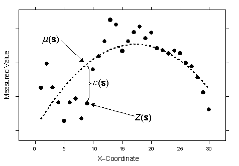
Z(s) = µ(s) + ε(s),

where µ(s) is some deterministic function. For example, in the following figure, which has the same data that was used for ordinary kriging concepts, the observed data is given by the solid circles.

A second-order polynomial is the trend—long dashed line—which is µ(s). If you subtract the second-order polynomial from the original data, you obtain the errors, ε(s), which are assumed to be random. The mean of all ε(s) is 0. Conceptually, the autocorrelation is now modeled from the random errors ε(s). Of course, you could have fit a linear trend, a cubic polynomial, or any number of other functions. The figure above looks just like a polynomial regression from any basic statistics course. In fact, that is what universal kriging is. You are doing regression with the spatial coordinates as the explanatory variables. However, instead of assuming the errors ε(s) are independent, you model them to be autocorrelated. The advice is the same as for ordinary kriging: there is no way to decide, based on the data alone, on the proper decomposition.

Universal kriging can use either semivariograms or covariances (which are the mathematical forms you use to express autocorrelation), use transformations, and allow for measurement error.