Geostatistical Analyst のライセンスで利用可能。
How the realizations are generated
Gaussian Geostatistical Simulations works by first creating a grid of randomly assigned values drawn from a standard normal distribution (mean = 0 and variance = 1). The covariance model (from the semivariogram specified in the simple kriging layer, which is required as input for the simulation) is then applied to the raster. This ensures that raster values conform to the spatial structure found in the input dataset. The resulting raster constitutes one unconditional realization, and many more can be produced using a different raster of normally distributed values each time. Details of this method may be read in Dietrich and Newsam (1993).
If conditional simulation has been selected, the unconditional rasters are conditioned via kriging. This process uses the kriged estimate (prediction) at each location to ensure that the simulated values honor the input data values and that, on average, the kriged predictions are replicated. Details of conditioning the realizations using kriging may be read in Journel (1974).
However, if the simple kriging model includes measurement error, the input data values will not be honored (in the simple kriging layer or in the simulated realizations). In addition to this, the Gaussian Geostatistical Simulations tool has been implemented to use a continuous (or smooth) search neighborhood that avoids discontinuities in the simulated surfaces due to changes in the local neighborhood used in kriging. Details can be found in Aldworth (1998) and Gribov and Krivoruchko (2004).
To read more on geostatistical simulation concepts and for examples of conditional and unconditional simulation, refer to the help section on key concepts of geostatistical simulation.
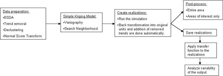
A general workflow for Gaussian geostatistical simulation involves preparing the data, creating the realizations, back transforming the results into original units, and postprocessing the results and/or using the results as input to a transfer function (model) to assess variability in the model's output. This process is represented in the following figure:

Checking simulation output
Realizations should be checked to confirm the following:
- The output values, their spatial patterns, and locations are reasonable.
- The simulated data's histogram reproduces the input data's histogram, on average.
- The simulated data's semivariograms reproduce the input data's semivariogram, on average.
- For conditional simulation, the input data values are honored (unless the simple kriging model includes measurement error).
Postprocessing
Once the realizations have been produced, they are usually postprocessed to obtain summaries of the results. The Gaussian Geostatistical Simulations tool allows several postprocessing options, which can be performed on the entire spatial extent of the rasters or on areas of particular interest. These areas are defined by specifying a polygon feature class in the Input statistical polygons option of the tool. Output is similar in both cases: postprocessing the entire rasters produces summary rasters, while postprocessing on polygonal areas produces a polygon output feature class that contains summary statistics for each polygon.
Postprocessing the entire raster extent
- Output rasters include the minimum value generated for each location (cell), as well as the maximum, mean, standard deviation, first quartile, median (second quartile), and third quartile. Additionally, you can specify a quantile that will return a value corresponding to that quantile, based on the distribution of values simulated at each cell. You can also specify a threshold value, which will return the percentage of simulated values that exceed the threshold for each cell.
- Note that the extent to be postprocessed can be limited by specifying a bounding polygon or a set of points (in this case, a convex hull is generated and used as a bounding polygon). Values are only simulated within the bounding polygon.
Postprocessing for areas of interest
- When polygon areas of interest are specified, the output for each polygon automatically includes the summary statistics described in the table below. Additionally, you can specify a quantile value and a threshold value (as when postprocessing the entire raster extent). Output generated when these options are selected is also described in the table.
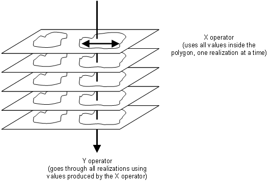
- Summary output for the polygons is calculated using operators such as those represented in the figure below. The X operator utilizes all the values that fall within the polygon and calculates a value for each realization. The Y operator uses values from all the realizations. Inputs for the Y operator are the values for the polygonal areas of each realization, calculated by the X operator.

The meanings of the fields in the output feature class are listed in the following table.
| Field name | Description |
|---|---|
MIN | Minimum value of any cell in all the realizations that fall within the polygon. |
MAX | Maximum value of any cell in all the realizations that fall within the polygon. |
MEAN | Mean of all the cells in all the realizations that fall within the polygon. |
STDDEV | Standard deviation of all the cells in all the realizations that fall within the polygon. |
QUARTILE1 | First quartile value of all the cells in all the realizations that fall within the polygon. |
MEDIAN | Median value of all the cells in all the realizations that fall within the polygon. |
QUARTILE3 | Third quartile value of all the cells in all the realizations that fall within the polygon. |
QUANTILE | Value corresponding to a user-specified quantile for all the cells in all the realizations that fall within the polygon. |
P_THRSHLD | Percentage of cells that exceeded a user-specified threshold value, based on all the cells in all the realizations that fall within the polygon. |
X_Y | The X function is applied to the values of the cells that fall within the polygon, one realization at a time. This process is equivalent to running the Zonal Statistics tool using the polygon as a zone and one realization at a time as the value grid. The Y function is applied to the values produced by the X function.
|
CELL_COUNT | The number of cells that fall within the polygon. If the cell center falls within the polygon, that cell is deemed to be in the polygon. A negative count indicates that part of the polygon falls outside the extent of the simulated raster and/or part of the polygon falls outside the clipping boundary. The negative number itself indicates the total number of cells that fall within the polygon. |
SOURCE_ID | The object or feature ID of the input polygon feature class. |
For both the bounding polygon and the polygon areas of interest options, raster cells are deemed to be inside the polygons if the center of the cell falls inside the polygon's boundary.
An example of conditional simulation and postprocessing output
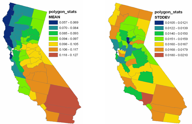
The following figure shows the results of conditional simulation with polygon postprocessing of the output. The maps show the mean and standard deviation of 100 realizations of ozone values for each county in California. These mean and standard deviation values could be used, for example, in epidemiological studies where the occurrence of a disease needs to be compared with the average ozone value for each county.

References and further reading
Aldworth, J. 1998. Spatial Prediction, Spatial Sampling, and Measurement Error. Ph.D. Thesis, Iowa State University. 186.
Chiles, J. P., and P. Delfiner. 1999. Geostatistics: Modeling Spatial Uncertainty. New York: John Wiley & Sons, 449–471.
Deutsch, C. V., and A. G. Journel. 1998. GSLIB Geostatistical Software Library and User's Guide, 2nd edition. New York: Oxford University Press, 119–141.
Dietrich, C. R., and G. N. Newsam. 1993. "A Fast and Exact Method for Multidimensional Gaussian Stochastic Simulations." Water Resources Research 29 (8): 2861–2869.
Goodchild, M. F., B. O. Parks, and L. T. Steyaert. 1993. Environmental Modeling with GIS. New York: Oxford University Press, 432–437.
Gribov, A., and K. Krivoruchko. 2004. "Geostatistical Mapping with Continuous Moving Neighborhood." Mathematical Geology 36 (2): 267–281.
Journel, A. G. 1974. "Geostatistics for Conditional Simulation of Ore Bodies." Economic Geology 69: 673–687.
Leuangthong, O., J. A. McLennan, and C. V. Deutsch. 2004. "Minimum Acceptance Criteria for Geostatistical Realizations." Natural Resources Research 13 (3): 131–141.