Geostatistical Analyst のライセンスで利用可能。
Simulation concepts
Simulation is broadly defined as the process of replicating reality using a model. In geostatistics, simulation is the realization of a random function (surface) that has the same statistical features as the sample data used to generate it (measured by the mean, variance, and semivariogram). Gaussian geostatistical simulation (GGS), more specifically, is suitable for continuous data and assumes that the data, or a transformation of the data, has a normal (Gaussian) distribution. The main assumption behind GGS is that the data is stationary—the mean, variance, and spatial structure (semivariogram) do not change over the spatial domain of the data. Another key assumption of GGS is that the random function being modeled is a multivariate Gaussian random function.
GGS offers an advantage over kriging. Because kriging is based on a local average of the data, it produces smoothed output. GGS, on the other hand, produces better representations of the local variability because it adds the local variability that is lost in kriging back into the surfaces it generates. The variability that GGS realizations add to the predicted value at a particular location has a mean of zero, so that the average of many GGS realizations tends toward the kriging prediction. This concept is illustrated in the figure below. Different realizations are represented as a stack of output layers, and the distribution of values at a particular coordinate is Gaussian, with a mean equal to the kriged estimate for that location and a spread that is given by the kriging variance at that location.
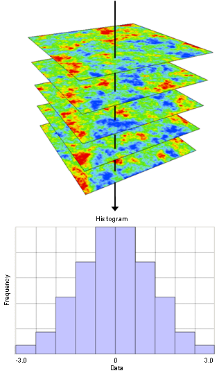
The Extract Values To Table tool can be used to produce the data for the graph illustrated in the figure above, as well as aid in post-processing the output generated by GGS.
Increased use of GGS follows a trend in geostatistical practice that emphasizes the characterization of uncertainty for decision and risk analysis, rather than producing the best unbiased prediction for each unsampled location (as is done with kriging), which is more suited to showing global trends in the data (Deutsch and Journel 1998, Goovaerts 1997). Simulation also overcomes the problem of conditional bias in kriged estimates (high-value areas are typically underpredicted, while low-value areas are usually overpredicted).
Geostatistical simulation generates multiple, equally probable representations of the spatial distribution of the attribute under study. These representations provide a way to measure uncertainty for the unsampled locations taken all together in space, rather than one by one (as measured by the kriging variance). Moreover, the kriging variance is usually independent of the data values and generally cannot be used as a measure of estimation accuracy. On the other hand, estimation accuracy can be measured by building distributions of estimated values for unsampled locations using multiple simulated realizations that are built from a Simple Kriging model using input data that is normally distributed (that is, data that either is normally distributed or has been transformed using a normal score or other type of transformation). These distributions of uncertainty are key to risk assessment and decision analysis that use the estimated data values.
GGS assumes that the data is normally distributed, which rarely occurs in practice. A normal score transformation is performed on the data so that it will follow a standard normal distribution (mean = 0 and variance = 1). Simulations are then run on this normally distributed data, and the results are back-transformed to obtain simulated output in the original units. When Simple kriging is performed on normally distributed data, it provides a kriging estimate and variance that fully define the conditional distribution at each location in the study area. This allows one to draw simulated realizations of the random function (the unknown, sampled surface) knowing only these two parameters at every location, and is the reason that GGS is based on a Simple kriging model and normally distributed data.
The Gaussian Geostatistical Simulations tool allows two types of simulation:
- Conditional simulation honors the data values (unless measurement error has been included in the kriging model). Some differences between measured and simulated values for sample locations may occur because simulation generates values at grid cell centers, which may not correspond exactly to the location of the sample points. Conditional simulation also replicates the mean, variance, and semivariogram of the data, on average (that is, averaged over many realizations). The simulated surfaces look like kriging prediction maps but show more spatial variability.
- Unconditional simulation does not honor the data values, but does replicate the data's mean, variance, and semivariogram (on average). The simulated surfaces show spatial structure that is similar to a kriged map, but high- and low-value areas will not necessarily occur where high- and low-data values exist in the input data.
Examples of simulation
Example 1
Air quality is an important health concern in many cities and areas around the world. Within the United States, Los Angeles is known for having poor air quality, and an extensive monitoring network collects data on ozone, particulate matter, and other contaminants on a subdaily basis. This air quality data is reported as the concentration of each contaminant, as well as the number of days per year in which a contaminant exceeded the state and federal air quality standards (https://www.arb.ca.gov/html/ds.htm). While both measures allow partial assessments of the exposure risks of living in a particular area, the number of days per year that the critical thresholds were exceeded can be used to make interpolated maps showing probabilities of threshold exceedance.
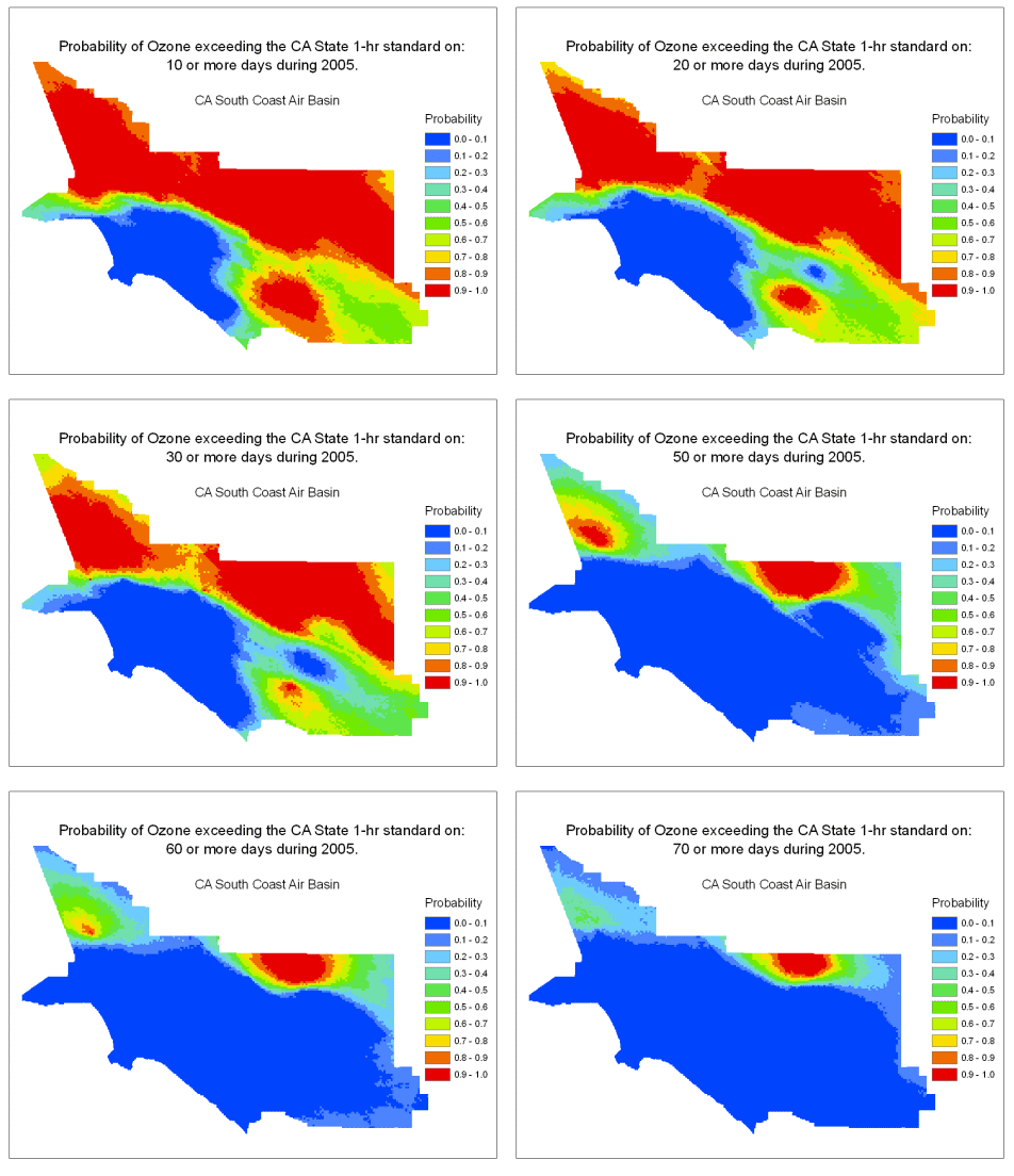
In this example, the number of days that the California State ozone threshold was exceeded at each monitoring station during 2005 was examined, and a semivariogram was fitted to it. Conditional simulation was used to produce multiple realizations. Each realization is a map of the number of days that the contaminant exceeded the threshold value during 2005. The realizations were then postprocessed to estimate probabilities that the contaminant exceeded the state threshold more than 10, 20, 30, 40, 50, 60, and 70 days per year (the maximum recorded by any station was 80 days during which the threshold was exceeded). The animation below shows the resulting maps for ozone in the South Coast Air Basin, which includes Los Angeles and inland cities. Air quality near the coast is considerably better than inland areas, mainly due to winds blowing predominantly from west to east in this region.
Maps such as these are useful in prioritizing abatement strategies, for studying the relationships between health and environmental quality, and for the population to make decisions on where to live by providing information that can help them answer questions such as How much pollution am I willing to tolerate? and How much pollution do I have to tolerate to live in a certain area?
Example 2
There are many applications in which spatially dependent variables are used as input for models (for example, flow simulation in petroleum engineering). In these cases, uncertainty in the model's results is evaluated by producing a number of simulations using the following procedure:
- 1. A large number of equally probable realizations are simulated for the variable.
- 2. The model (generally termed a transfer function) is run using the simulated variable as input.
- 3. The model runs are summarized to evaluate variability in the model's output.
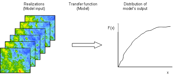
The statistics of the output provide a measure of the uncertainty of the model.
A real-world example of the procedure described above is the study conducted to open the Waste Isolation Pilot Plant (WIPP) in southeastern New Mexico as a storage facility for transuranic waste (https://www.wipp.energy.gov/).
Scientists were evaluating salt deposits more than 2,000 feet below the earth's surface as a potential storage facility for the waste material. However, the deposits lie just above an aquifer, and there was concern that groundwater might transport waste that could leak from the site. To demonstrate that the WIPP was safe, scientists had to convince the U.S. Environmental Protection Agency that the velocity of groundwater flowing through the aquifer is low enough that contamination of the surrounding environment is extremely unlikely.
Transmissivity values determine the rate of water flow through an aquifer, and several such values were obtained for the aquifer near the proposed WIPP site. Groundwater flow is modeled using hydrologic equations that are solved numerically and require transmissivity values predicted on a regular grid. If kriging estimates of transmissivity were used, the transmissivity values would be based on (weighted) averages of neighboring transmissivity values, and the modeled groundwater travel time would be based only on these average values. Because kriging produces smoothed maps, areas of extremely high and low transmissivity values would be missing from the interpolated surfaces. To analyze the risk correctly, the scientists had to consider the worst possible scenario and thus needed to produce an entire probability distribution of travel time values. With this, they could use the lower tail values of the groundwater travel time distributions (corresponding to extremely high flow velocity), and not the average travel times, to evaluate the suitability of the WIPP. Conditional simulations were used to produce the probability distributions of time travel values.
The possibility that waste products might be transported by groundwater was only one of many different human-risk scenarios considered in evaluating suitability of the WIPP. Complex risk analysis played a large part in assessing the WIPP for nuclear waste disposal and convincing the public and government regulators of its suitability. Following more than 20 years of scientific study, public input, and regulatory struggles, the WIPP began operations on March 26, 1999.
How many realizations should be generated?
Results from simulation studies should not depend on the number of realizations that were generated. One way to determine how many realizations to generate is to compare the statistics for different numbers of realizations in a small portion of the data domain (a subset is used to save time). The statistics tend toward a fixed value as the number of realizations increases. The statistics examined in the example below are the first and third quartiles, which were calculated for a small region (subset) of simulated elevation surfaces (in feet above sea level) for the state of Wisconsin, USA.
The top graph shows fluctuations in elevation for the first 100 realizations. The lower graph shows results for 1,000 realizations.
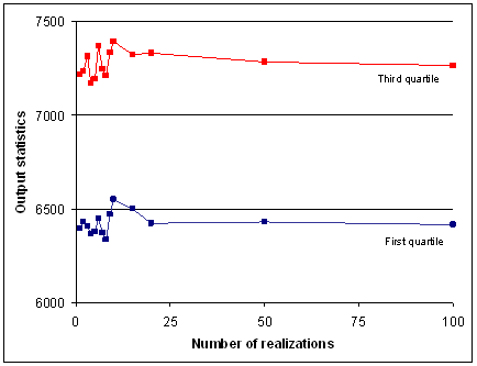
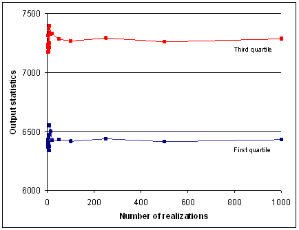
In this case, the values stabilize after about 20 simulations. In many cases, at least 100 realizations are run to provide sufficient information to determine the mean and probabilities of exceeding a threshold value. A larger number of realizations allows higher degrees of certainty in the summary statistics and model output variables but requires more computing time.
To learn more about how Gaussian Geostatistical Simulation has been implemented in ArcGIS, please refer to the help section How Gaussian Geostatistical Simulations work.
References
Deutsch, C.V., and A. G. Journel. 1998. GSLIB Geostatistical Software Library and User's Guide. 2nd Ed. Oxford University Press, New York, pages 119–122.
Goovaerts, P. 1997. Geostatistics for Natural Resource Evaluation. Oxford University Press, New York, pages 369–376.