Geostatistical Analyst のライセンスで利用可能。
Simple kriging assumes this model:
Z(s) = µ + ε(s)- where µ is a known constant
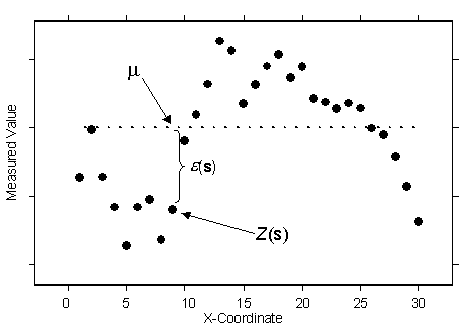
For example, in the following figure, which uses the same data as for ordinary kriging and universal kriging concepts, the observed data is given by the solid circles:

The known constant, represented by the dotted line, is µ. This can be compared to ordinary kriging. For simple kriging, because you assume that you know µ exactly, you also know ε(s) exactly at the data locations. For ordinary kriging, you estimated µ, so you also estimated ε(s). If you know ε(s), you can do a better job of estimating the autocorrelation than if you are estimating ε(s). The assumption that you will know the exact mean µ is often unrealistic. However, sometimes it makes sense to assume that a physically based model gives a known trend. Then you can take the difference between that model and the observations, called residuals, and use simple kriging on the residuals, assuming the trend in the residuals is known to be zero.
Simple kriging can use either semivariograms or covariances (which are the mathematical forms you use to express autocorrelation), use transformations, and allow for measurement error.