Find the best routes to service paired orders

Available with Network Analyst license.

In this exercise, your goal is to find the best routes for a fleet of vans to transport people who would otherwise not have access to transportation from their homes to hospitals for medical appointments. You will accomplish this by solving a vehicle routing problem (VRP) analysis using order pairs, which relate and sequence two orders (stops) so that the vans will pick up riders and take them to their destinations. Using other features of the VRP analysis layer, you will also ensure that additional requirements are met. For instance, enter a maximum transit time for order pairs so that riders don't spend too much time in transit; use time windows on orders so that riders are not late for their appointments. Some riders require wheelchairs; you will use specialties to match those riders with vans that have wheelchair lifts. Once the routes are determined, publish the routes to ArcGIS.com so the drivers can access them through Navigator.

Note:

This tutorial can be completed using as the network data source either the designated tutorial network dataset, ArcGIS Online, or an ArcGIS Enterprise routing service published using a network dataset that covers the geography of the input data of the analysis. If you use ArcGIS Online, credits will be consumed. Learn more about network analysis with a service.

Get the data

The data for this tutorial is available for download.

1. Go to the data download page.
2. Click the Download button, and save the file locally.
3. Unzip the downloaded file.

Create a map

Complete the following steps to create a map:

1. Start ArcGIS Pro.
2. Create a new project by clicking the Map template. Optionally, change the name of your project and location.

   A new project with a map appears.

Add the tutorial data to the project

A network dataset is an intelligent model of the road system. It contains not only the location and attributes of roads but also information about how roads relate to one another, such as which roads are connected, which turns between connected roads are allowed or prohibited, and other information that affects what travel paths are possible and how long travel takes. The VRP solver references the network dataset to determine the shortest path between stops.

Note:

If you perform an analysis using ArcGIS Online, the solver references a high-quality, worldwide network dataset stored in the ArcGIS Online cloud and uses ArcGIS Online credits. You can also use your own network dataset stored locally on your machine or use ArcGIS Enterprise to publish routing services using your own network dataset and configure the services with your enterprise portal to consume them from ArcGIS Pro.

In this set of steps, add a network dataset to the map.

1. In the Catalog pane, which is on the right side of the application by default, right-click Folders and choose Add Folder Connection .

   The Add Folder Connection dialog box appears.

2. Browse to the folder where you placed the tutorial data, double-click Network Analyst, and click Tutorial to select the folder.
3. Click OK.

   A connection to the Tutorial folder is created.

Next, add one of the network datasets contained in the folder to the map.

Note:

You do not need to add the network dataset to the map if you intend to use ArcGIS Online or an ArcGIS Enterprise routing service as the network data source.

4. In the Catalog pane, expand Folders > Tutorial > SanFrancisco.gdb > Transportation.
5. Drag Streets_ND, which has a network dataset icon , onto the map.

   The network dataset is added to the Contents pane and to the map.

6. If needed, right-click Streets_ND in the Contents pane and choose Zoom To Layer to view the San Francisco area.

   By default, network datasets built with traffic data show traffic conditions for the current time when they are added to the map. This network dataset includes historical traffic, so you are seeing typical traffic conditions for the current time and day of the week. Not all roads in this network dataset include traffic, so only the ones that do are shown by default.

   The area covered by the network dataset is where you can perform network analyses.

   Viewing the network dataset isn't required to perform an analysis, so next, you will hide it.

7. In the Contents pane, uncheck Streets_ND to display the basemap only.
Add the points that represent the depot locations for the vans on the map.
8. In the Catalog pane, browse to Tutorial > SanFrancisco.gdb > Analysis.
9. In the Catalog pane, right-click the CentralDepots layer and choose Add to Current Map.

   Note:

   You can also add a layer to the map by dragging it from the Catalog pane onto the map.

   The CentralDepots layer is added to the Contents pane and to the map.

Create the Vehicle Routing Problem layer

A Vehicle Routing Problem (VRP) layer provides the structure and properties needed to set up and solve multiple vehicle routing problems. It also contains the results after solving.

1. On the Analysis tab, in the Workflows group, click Network Analysis > Vehicle Routing Problem .

   The VRP layer is added to the Contents pane. It includes several sublayers that hold the inputs and outputs of the analysis.

   The route is referencing the San Francisco network dataset because the network was in the Contents pane when the route layer was created.

   Note:

   To see or change the network data source that is used to create the network analysis layer, on the Analysis tab, in the Workflows group, you can click the Network Analysis drop-down menu and look under Network Data Source.

2. In the Contents pane, click Vehicle Routing Problem to select the group layer.

   The VRP Layer tab appears.

3. Click VRP Layer to see the settings on the tab.
   

   You'll use these controls to define the VRP model you want to generate.

   Tip:

   The VRP Layer tab appears only when you select a VRP layer in the Contents pane. Also, If you have multiple VRP layers, you can change the settings of the layers individually or select the multiple layers to edit the settings for all the selected layers if they share the same network data source.

Add orders

A spreadsheet is provided with the tutorial data. It contains information about each patient, including their name and home address, the name and address of the hospital they must be taken to, the time window within which the patient must be picked up, and so on. The following table describes the fields in the spreadsheet:

Attribute	Description
OrderName1	The name of the patient needing transportation
PatientAddress	The location where the patient will be picked up
OrderName2	A unique name for the destination
HospitalAddress	The location where the patient has the appointment
PickFrom	The earliest time the patient may be picked up from PatientAddress
PickTo	The latest time the patient may be picked up from PatientAddress
TotalPassengers	The total number of passengers to be picked up
MaxTransitTime	The maximum time the patient can spend in the van
SpecialityNames	Specifies the special needs that are required by the passenger, for example, a wheelchair

In this case, the passengers and hospital visits are related to each other, since each passenger must visit a predetermined hospital. You can model this scenario with order pairs by loading both patient and hospital locations into the Orders network analysis class and relating them with new order pair objects.

In the following steps, you will geocode the patient and hospital addresses and load the resulting points as orders:

1. In the Catalog pane, browse to the tutorial data location, find the OrderPairs.xls file and double-click it.

   The OrderPairs.xls file expands, and you'll see a table called Patients$.

Note:

An error message appears if the required Microsoft driver is not installed. Learn more about installing the drivers to work with Microsoft Excel files.
2. Right-click the Patients$ table and click Geocode Table from the context menu.

   The Geocode Table guided workflow pane appears. The opening page is a description of steps you will go through.

3. Click the Start button.
4. Click the Browse button next to the Input Locator parameter, browse to the saved location of the tutorial data, and select SanFranciscoLocator.loc.
5. Click OK.
6. Click Next.
7. For the question starting with "How is your data structured?", select One field from the drop-down list.
   
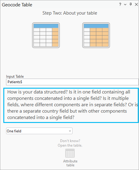
8. Click Next.
9. In the Data Field drop-down list, select the PatientAddress field, and click Next.

   You will first geocode the patients' home addresses.

10. For the Output field name, ensure that it lists Patients_Geocoded as the new feature class name.
11. Click Next.
12. Do not update anything in the Limit by Category step. Click Finish.
13. Review the inputs in the Geocode Table geoprocessing tool and click the Run button at the bottom of the pane.

    

14. Click No on the Geocoding Completed pop-up.

    You do not need to start the rematch process, since the address names were matched perfectly. In your own workflows, going through rematch may be necessary to clean up some of the address information.

15. Repeat steps 1 through 13 with the following changes to geocode the hospital locations for the patients' appointments:
    • In step 8, select HospitalAddress.
    • In step 9, change the Output name field to DestinationHospitals_Geocoded by clicking the browse button and type DestinationHospitals_Geocoded in the Name text box. Click Save.

    Tip:

    You can update the Geocode Table geoprocessing tool with the above values and rerun the tool without going back through the whole guided workflow.

16. In the Contents pane, uncheck the two geocoding result layers so they are not visible in the map display.

    In the next steps, you'll load these layers into the Orders network analysis class.

17. On the VRP Layer tab, in the Input Data group, click Import Orders.

    The Add Locations window appears.

18. Ensure Input Network Analysis Layer is set to Vehicle Routing Problem and Sub Layer is set to Orders.
19. Click the drop-down arrow for Input Locations and choose Patients_Geocoded. This is the point feature class you made in the previous steps that was added to the map automatically.
20. Under Field Mappings, choose Name from Property and select USER_OrderName1 in the Field Name parameter.
This indicates that the USER_OrderName1 field in the feature class should be mapped to the Name field when importing Orders.
21. Map the following fields if they are not automatically mapped:

    • Description > USER_PatientAddress
    • TimeWindowStart > USER_PickFrom
    • TimeWindowEnd > USER_PickTo
    • PickupQuantity_1 > USER_TotalPassengers

22. Under Field Mappings, choose ServiceTime from Property and type 2 in the Default Value parameter.

    All patient address locations that are loaded will have a Service Time Value of 2 to account for the average time (in minutes) that is taken for passengers to board the van.

23. Under Field Mappings, choose MaxViolationTime from Property and type 0 in the Default Value parameter.

    By setting all the MaxViolationTime properties to zero, the VRP solver will only search for routes that visit the orders within their time windows.

24. Leave the default settings for the rest of the parameters and click the OK button.

A total of 15 records are added in the Orders attribute table and displayed on the map.

25. Repeat steps 16 through 18 with the following changes:
• In step 18, choose DestinationHospitals_Geocoded.
• Make the following field mappings:
  • Name > USER_OrderName2
  • Description > USER_HospitalAddress
  • DeliveryQuantity_1 > USER_TotalPassengers

Note:

The value for the Name attribute must be unique in the Orders network analysis class. In this case, there are many patients who need to visit the same hospital. So if the hospital addresses were used to derive the value of the Name attribute for Orders, the VRP solver would return error messages, as there would be duplicate Name values.
26. Leave the default settings for the rest of the parameters and click the OK button.

A total of 15 records are added in the Orders attribute table and displayed on the map.

Add order pairs

The passengers must be taken to a predetermined hospital. By adding objects to the Order Pairs network analysis class, you can add the information that specifies which hospital the patients have to be taken to and the maximum time the patients can sit in the van during a one-way trip.

1. On the VRP Layer tab, in the Input Data group, click Import Order Pairs from the drop-down list of import options.

   

   The Add Locations window appears.

   You have previously used this tool to load orders from a feature class. Now you will use it to load data into the OrderPairs table from an Excel file.

2. Ensure Input Network Analysis Layer is set to Vehicle Routing Problem and Sub Layer is set to Order Pairs.
3. Click the browse button next to the Input Locations field and browse to the location of the tutorial data to select the Patients$ table from within the OrderPairs.xls file.
4. Verify that the following field mappings have automatically populated:
• FirstOrderName > OrderName1
• SecondOrderName > OrderName2
• MaxTransitTime > MaxTransitTime
5. Leave the default settings for the rest of the parameters and click the OK button.

A total of 15 records are added in the OrderPairs table.

Add depots

The logistics company operates vans from three depots whose locations are shown in the CentralDepots feature layer you have previously added to the map. You will now add these point features to the Depots network analysis class.

1. On the VRP Layer tab, in the Input Data group, click Import Depots.

   The Add Locations window appears.

2. Ensure Input Network Analysis Layer is set to Vehicle Routing Problem and Sub Layer is set to Depots.
3. Click the drop-down arrow for Input Locations and choose CentralDepots.
4. Under Field Mappings, choose Name from Property, and ensure Name is automatically mapped in the Field Name parameter.
5. Leave the default settings for the rest of the parameters and click the OK button.

Three records are added to the Depots attribute table and displayed on the map.

Add routes

The logistics company has three vans, each with a maximum capacity of six passengers. The vans start and return to the depots after completing all the trips. One of the vans that operates within the downtown area has a lift to provide easy access for wheelchairs.

You will add three routes, one for each van. In this section, you will add the routes using the Routes attribute table. Other options are to use the Add Locations tool to import a table that you have already created or to use the Add Vehicle Routing Problem Routes geoprocessing tool, which will create a set of routes with the same parameters. In this case, you have enough settings per route that the quickest method will be to enter the values directly in the table.

1. In the Contents pane, right-click Routes and select Attribute Table from the context menu.

   The attribute table appears with the input and output fields for each route.

2. Click the Click to add new row button to add information for the three routes as below:

   Name	StartDepotName	EndDepotName	Capacity_1
   Downtown	Downtown Depot	Downtown Depot	6
   North Bay	North Bay Depot	North Bay Depot	6
   East Bay	East Bay Depot	East Bay Depot	6

   

3. Click the Edit tab, and in the Manage Edits group, click the Save button .
4. Click Yes on the Save Edits dialog box.
5. Close the Routes attribute table.

Add specialties

Some of the patients being picked up are in a wheelchair, but only one of the vans has a lift to provide easy access into and out of the vehicle for these patients. You will therefore set up a specialty to indicate that these patients need support that is only provided by that route. If you look at the Excel document that was provided with the tutorial data, you will see that three patients need wheelchair accessibility: Tony, Tim, and Bill. Also, the downtown route is the only van with the wheelchair lift capability. In the next set of steps, you will add values in the Order Specialties and Route Specialties attribute tables to indicate this information.

First, you will enter the order specialties information.

1. In the Contents pane, right-click Order Specialties and select Open from the context menu.

   The attribute table appears, and you can enter the information about each order with a specialty.

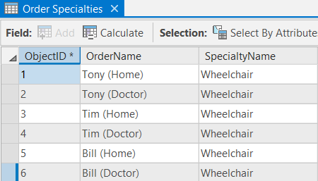
2. Click the Click to add new row button to add information, as shown below:

   OrderName	SpecialtyName
   Tony (Home)	Wheelchair
   Tony (Doctor)	Wheelchair
   Tim (Home)	Wheelchair
   Tim (Doctor)	Wheelchair
   Bill (Home)	Wheelchair
   Bill (Doctor)	Wheelchair

   

3. Click the Edit tab, and in the Manage Edits group, click the Save button .
4. Click Yes on the Save Edits dialog box.
5. Close the Order Specialties attribute table.
Now you will enter the route specialties information.
6. In the Contents pane, right-click Route Specialties and select Open from the context menu.

   The attribute table appears, and you can enter the information about each route that can serve a specialty.

7. Click the Click to add new row button.
8. For RouteName, enter Downtown.
9. For SpecialtyName, enter Wheelchair.
10. Click the Edit tab, and in the Manage Edits group, click the Save button .
11. Click Yes on the Save Edits dialog box.
12. Close the Route Specialties attribute table.

Add route zones

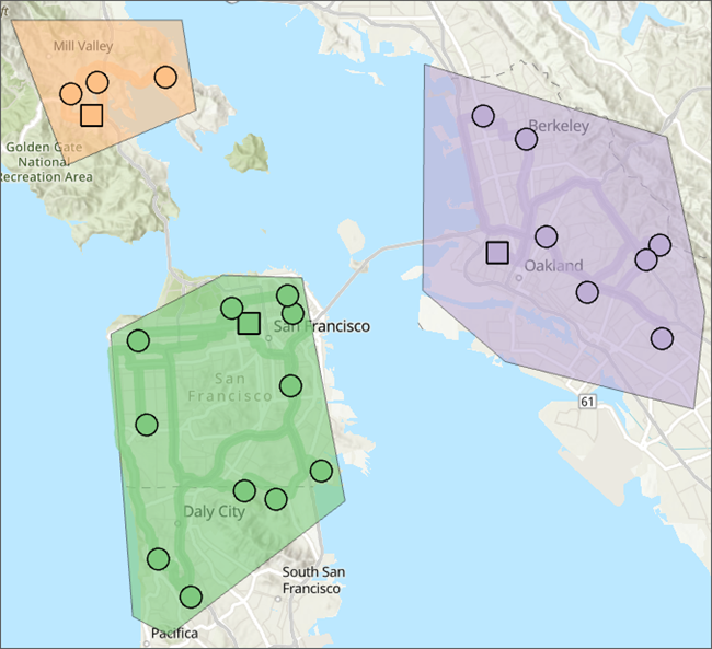
The three vans used by the company are only licensed to service orders in a predetermined area. You will add route zones and associate them with the vans or routes.

In this section, you will draw the boundaries of these zones using the Create Features pane; however, if you have zones already digitized, they can be imported using the Add Locations geoprocessing tool.

1. On the VRP Layer tab, in the Input Data group, click Create Features .

   The Create Features pane appears, showing the templates for the feature classes associated with the selected VRP layer.

2. In the Create Features pane, select Vehicle Routing Problem : Route Zones.
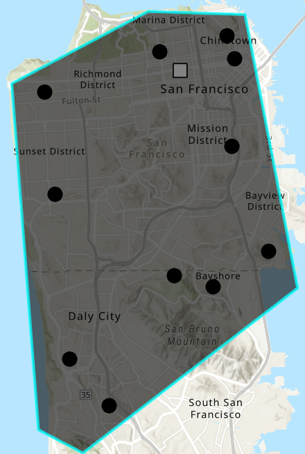
3. On the map display, digitize a polygon that roughly covers the downtown area, as shown below.

   

4. In the Contents pane, right-click Route Zones and select Attribute Table from the context menu.

   The attribute table appears, and you can enter the information about the route zone you just created.

5. Double-click in the first row under RouteName to edit the value and type Downtown.

   This is the name of the route associated with this route zone.

6. Ensure that the IsHardZone value is set to True.

   The van can't service orders that are outside the route zone. Setting this value to True ensures that the van is only assigned orders that are within the route zone.

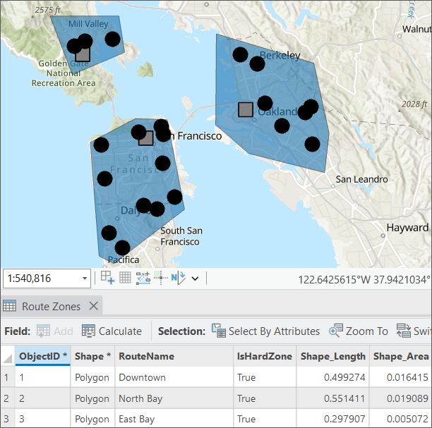
7. Repeat steps 3 through 6 to add two more route zones: one for the North Bay and the other for the East Bay.

   

8. Click the Edit tab, and in the Manage Edits group, click the Save button .
9. Click Yes on the Save Edits dialog box.
10. Close the Route Zones attribute table.

Set the properties for the vehicle routing problem analysis

Next, you will specify the properties for your vehicle routing problem analysis.

1. On the VRP Layer tab, in the Travel Settings, ensure the Mode is set to Driving Time.

   This travel mode encapsulates several settings such, as U-turn policy, restricted street policies, and values to use for time and distance costs.

2. In the Travel Settings group, ensure that Time Field Units is set to Minutes and Distance Field Units is set to Miles.
3. In the Default Date group, select Day of Week from the Default Date Type drop-down list.
4. From the resulting drop-down list with days of the week, select Monday.
5. In the Output Geometry group, select Along Network from the Output Geometry Linear Shape Type drop-down list.

   Note:

   The output geometry options only affect the display of the routes, not the results determined by the VRP solver.

Since you created route zones and associated them with the routes, spatial clustering should be turned off.
6. In the Advanced group, click the Cluster drop-down menu and select Do Not Cluster

   If you choose to select Cluster, on solving the analysis, spatial clustering is automatically turned off and the following warning message is received once the solve is completed " Spatial clustering of orders is disabled when Route Zones is non-empty."

Run the analysis

Run the VRP analysis to determine the best route assignment.

1. On the VRP Layer tab, click Run .

   The VRP solver calculates the routes for each van. Each route begins at a depot, the van picks up one or more people if the time they spend on the van is less than the MaxTransitTime specified in the order pair, drops them at their hospital locations, continues to pick up and drop off other people, and returns to the depot at the end. The routes only service orders in their assigned route zones.

   

Open the Orders attribute table and see when the patients will be picked up and dropped of by looking at the ArriveTime field. Additionally, you can get the information about how long each route will take by looking at the TotalTime field in the attribute table of the Routes sublayer.

Note:

In the TimeWindowStart and TimeWindowEnd fields, 12/30/1899 is interpreted as "today". See dates and times for more information.